Finite-difference scheme

In the approximated dispersion relation (6), replacing S_z and S_x by the partial differential operators $i \frac{\partial}{\partial z} /\frac{\omega}{V_{P0}}$ and $i\frac{\partial}{\partial x}/\frac{\omega}{V_{P0}}$, we obtain a partial differential equation as follows:  

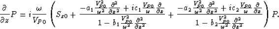$$\frac{\partial }{\partial z}P=i\frac{\omega}{V_{P0}}\left( S... ...{V_{P0}^2}{\omega^2}\frac{\partial^2}{\partial x^2} } \right)P.$$ (7)

Equation (7) can be solved by cascading as follows:

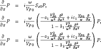$$\begin{eqnarray} \frac{\partial }{\partial z}P&=&i\frac{\omega}{V_{P0}}S_{z0}P, ... ...rac{V_{P0}^2}{\omega^2}\frac{\partial^2}{\partial x^2} } \right)P.\end{eqnarray}$$ (8) (9) (10)

Equation (8) can be solved by a phase-shift in the space domain. Let $P^n_i=P(\omega,n\Delta z,i\Delta x)$, where $\Delta x$ and $\Delta z$ are the grid size of finite-difference scheme. In equation (9), replacing the partial differential operators by the finite-difference operators as follows:

$$\frac{\partial }{\partial x}P(\omega,n\Delta z,i\Delta x)\approx\delta_xP^n_i= \frac{P_{i+1}^n-P_{i-1}^n}{2\Delta x}$$

and

$$\frac{\partial^2 }{\partial x^2}P(\omega,n\Delta z,i\Delta x... ... \delta_x^2P^n_i=\frac{P_{i+1}^n-2P_i^n+P_{i-1}^n}{\Delta x^2},$$

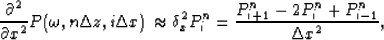
we can derive the following finite difference equation:  

$$\left(1+(\frac{ia_1\Delta z}{2}\frac{V_{P0}}{\omega}-b_1\fra... ...ega^2})\delta_x^2-\frac{c_1\Delta z}{2}\delta_x \right) P_i^{n}$$ (11)

Fourier analysis shows that the finite-difference scheme (11) is stable. Its computational cost is almost same as that of the finite-difference scheme for isotropic media. Equation (10) can be solved similarly.