Cost-efficient prestack exploding-reflector modeling

The independent modeling and imaging of all SODCIGs in a prestack image would be computationally expensive. However, several SODCIG can be modeled together, thus drastically reducing the number of independent experiment that must be modeled and imaged. The combinations of the several SODCIG can be expressed as the following summation:  

$$I_{j}\left(z_\xi,x_\xi,h_\xi\right) = \sum_{i \in A_j} I\left(z_\xi,x_\xi^{i},h_\xi\right),$$ (18)

where A_j is the set of SODCIGs combined for creating one single modeling experiment.

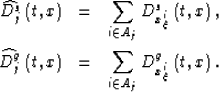
Because of the linearity of equations 12 and 13, the data computed by modeling the subset A_j can be expressed as the sum of the data sets obtained by modeling each $x_\xi^{i}$ independently; that is,

$$\begin{eqnarray} \widehat{D^s_j}\left(t,x\right) &=& \sum_{i \in A_j} D^s_{x_\... ...t,x\right) &=& \sum_{i \in A_j} D^g_{x_\xi^{i}}\left(t,x\right).\end{eqnarray}$$ (19) (20)

The result of migrating this combined data set can be written as follows:

$$\begin{eqnarray} \lefteqn{\widehat{I}_{j}\left(z_\xi,x_\xi,h_\xi\right)} \nonumb... ...xi'; \right) I\left(z_\xi',x_\xi^{k}-h_\xi',h_\xi'\right) \right].\end{eqnarray}$$ (21)

The first term in equation 22 is the desired result; that is, the image that we would obtain if we had independently modeled and imaged each SODCIG belonging to A_j, and summed the results. The second term in equation 22 represents the ``cross-talk'' between the SODCIGs; these artifacts are the unwanted consequence of combining SODCIGs before modeling in order to save computations.

The second term in equation 22 becomes easier to analyze in the special case when migration velocity is the same as the modeling velocity. The ``residual propagation'' operator $\Delta G$ thus approximates a delta function and equation 22 simplifies into:  

$${\widehat{I}_{j}\left(z_\xi,x_\xi,h_\xi\right)} \approx \sum... ...}+h_\xi,h_\xi\right) I\left(z_\xi,x_\xi^{k}-h_\xi,h_\xi\right).$$ (22)

In this case, the the cross-talks terms are given by the product of each SODCIG in A_j, shifted by the subsurface offset $h_\xi$, with all the other SODCIG in A_j, shifted by $-h_\xi$.If we assume that the SODCIGs have limited subsurface offset range because they are partially focused by migration, we can easily eliminate the cross-talks interference with the desired image in a window around zero subsurface offset by ensuring that the SODCIG belonging to A_j are sufficiently separated in space. The numerical examples in the next section demonstrates this point.

However, if the migration and modeling velocities are dissimilar, the shifted versions of the SODCIGs contributing to the cross-talk are distorted and shifted by the ``residual propagation'' operator $\Delta G$ (equation  22). This additional shift may increase, or decrease, the amount of interference of the cross talks with the desired image. The last example in the next section illustrates this point.

 

• Synthetic data examples