Diffracted multiple

Consider now a diffractor sitting at the water-bottom as illustrated in the sketch in Figure . The source- and receiver-side multiples are described by equations 2-4 as did the water-bottom multiple. In this case, however, the take-off angles from source and receiver are different even if the surface offset is the same as that in Figure . In fact, since the reflection is non-specular at the location of the diffractor, X_diff needs to be known in order for the receiver take-off angle to be computed. The traveltime of the diffracted multiple is given by  

$$t_m=\frac{1}{V_1}\left[3\sqrt{Z_{wb}^2+\left[\frac{X_{diff}-... ...t]^2}+\sqrt{\left[(m_D+h_D)-X_{diff}\right]^2+Z_{wb}^2}\right],$$ (21)

where Z_wb=Z_diff can be computed from the traveltime of the multiple for the zero subsurface offset trace (t_m(0)) by solving the quadratic equation in Z_wb² that results from setting h_D=0 in equation 21:

64Z_wb⁴-20V₁²t_m²(0)Z_wb²+(V₁⁴t_m⁴(0)-4V₁²t_m²(0)(m_D-X_diff)²)=0

 

mul_sktch5 Figure 7 Imaging of receiver-side diffracted water-bottom multiple from a diffractor sitting on top of a flat water-bottom. At the diffractor the reflection is non-specular. Notice that $m_D\ne m_\xi$.

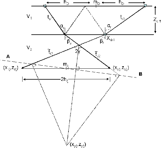The coordinates of the image point, according to equations 2-4 are given by

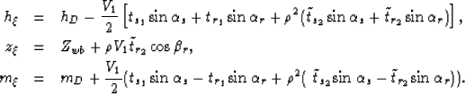$$\begin{eqnarray} h_\xi&=&h_D-\frac{V_1}{2}\left[t_{s_1}\sin\alpha_s+t_{r_1}\sin\... ...\rho^2(~\tilde{t}_{s_2}\sin\alpha_s-\tilde{t}_{r_2}\sin\alpha_r)).\end{eqnarray}$$ (23) (24) (25)

The traveltimes of the individual ray segments are given by

$$t_{s_1}=t_{s_2}=t_{r_2}=\frac{X_{diff}-(m_D-h_D)}{3V_1\sin\a... ...ox{and}\quad t_{r_1}=\frac{m_D+h_D-X_{diff}}{V_1\sin\alpha_r},$$ (26)

whereas the traveltimes of the refracted rays can be computed from equation 5:  

$$\tilde{t}_{s_2}=\frac{t_{s_2}(2\rho\cos\beta_r-\cos\alpha_s)... ...s\alpha_s)-t_{r_1}\cos\alpha_r}{\rho(\cos\beta_r+\cos\beta_s)}.$$ (27)

where, according to equations 9 and 10:  

$$\cos\beta_s=\sqrt{1-\rho^2\sin^2\alpha_s}\quad\mbox{and}\quad\cos\beta_r=\sqrt{1-\rho^2\sin^2\alpha_r}.$$ (28)

In order to express $h_\xi$, $z_\xi$ and $m_\xi$ entirely in terms of the data space coordinates, all we need to do is compute the sines and cosines of $\alpha_s$ and $\alpha_r$ which can be easily done from the sketch of Figure :

$$\sin\alpha_s=\frac{X_{diff}-(m_D-h_D)}{3\sqrt{((X_{diff}-(m_... ...pha_s=\frac{Z_{wb}}{\sqrt{((X_{diff}-(m_D-h_D))/3)^2+Z_{wb}^2}}$$

$$\sin\alpha_r=\frac{(m_D+h_D)-X_{diff}}{\sqrt{((m_D+h_D)-X_{d... ...\frac{Z_{wb}}{\sqrt{((m_D+h_D)-X_{diff})^2+Z_{wb}^2}}\quad\quad$$

Notice that the diffraction multiple does not migrate as a primary even if migrated with water velocity. In other words, even if $\rho=1$, $h_\xi\ne 0$.The only exception is when X_diff=m_D+h_D/2 since then the diffractor is in the right place to make a specular reflection and therefore is indistinguishable from a non-diffracted water-bottom multiple. In that case, $\alpha_r=\alpha_s$ (which in turn implies $\beta_r=\beta_s$) and from equations 5 and 6, $\tilde{t}_{r_2}=\tilde{t}_{s_2}=t_{s_2}$ and therefore equations 23-25 reduce to equations 14-16, respectively.

 

image2
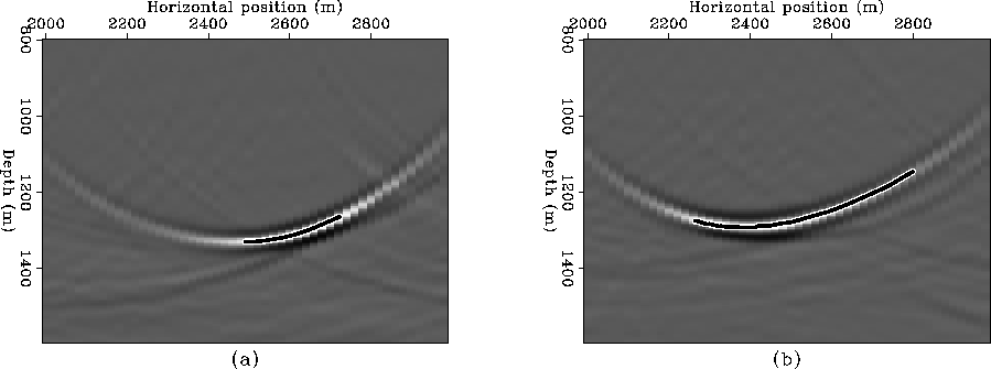
Figure 8 image sections at 0 and -400 m subsurface offset for a diffracted multiple from a flat water-bottom. The depth of the water-bottom is 500 m and the diffractor is located at 2500 m. The solid line represents image reflector computed with equations 24 and 25.

Figure  shows two subsurface-offset sections of a migrated diffracted multiple from a diffractor sitting on top of a flat reflector as in the schematic of Figure . The diffractor position is X_diff=2,500 m, the CMP range is from 2,000 m to 3,000 m, the offsets range from 0 to 2,000 m and the water depth is 500 m. The data were migrated with the same two-layer model described before. Panel (a) corresponds to zero subsurface offset ($h_\xi=0$) whereas panel (b) corresponds to subsurface offset of -400 m. Overlaid are the residual moveout curves computed with equations 24 and 25. Obviously, the zero subsurface offset section is not a good image of the water-bottom or the diffractor.

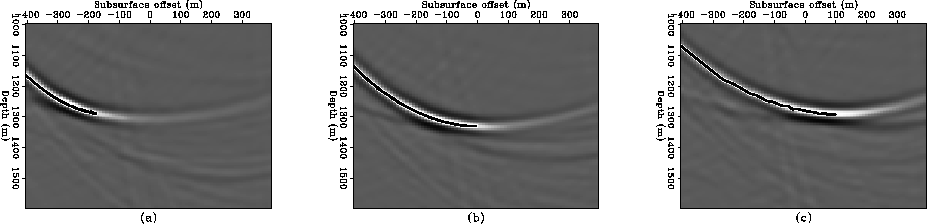
Figure  shows three SODCIGs taken at locations 2,300 m, 2,500 m and 2,700 m. Unlike the non-diffracted multiple, this time energy maps to positive or negative subsurface offset depending on the relative position of the CMP with respect to the diffractor. In ADCIGs the aperture angle is given by equation 11 which, given the geometry of Figure , reduces to  

$$\gamma=\frac{1}{2}\sin^{-1}\left[\beta_s+\beta_r\right]=\fra... ...\alpha_s}+\rho\sin\alpha_s\sqrt{1-\rho^2\sin^2\alpha_r}\right].$$ (29)

The depth of the image is given by equation 12,  

$$z_{\xi_\gamma}=z_\xi-h_\xi\tan\left(\frac{1}{2}\sin^{-1}\lef... ...s}+\rho\sin\alpha_s\sqrt{1-\rho^2\sin^2\alpha_r}\right]\right).$$ (30)

 

odcig2
Figure 9 SODCIGs from a diffracted multiple from a flat water-bottom at locations 2,300 m, 2,500 m and 2,700 m. The diffractor is at 2,500 m. The overlaid residual moveout curves were computed with equations 23 and 24.

Again, this equation shows that the diffracted multiple is not migrated as a primary even if $\rho=1$ (except in the trivial case X_diff=m_D+h_D/2 discussed before for which, since $\alpha_r=\alpha_s$, $\gamma=\beta_s=\beta_r$in agreement with equation 19 and so equation 30 reduces to equation 20).

 

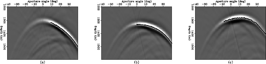
adcig2
Figure 10 ADCIGs corresponding to the SODCIGs in Figure . The overlaid curves are the residual moveout curves computed with equations 24 and 30.

Figure  shows the angle gathers corresponding to the SODCIGs of Figure . Notice the shift in the apex of the moveout curves.