


The correlated wavefield ![]() is not usable by the majority of
available reflection migration data tools. The source axis summation
explained above does not remove all of the potential time
delays. However, field data can still be migrated with a scheme that
includes separate extrapolation and correlation (for imaging)
steps. Artman and Shragge (2003) shows the applicability of
direct migration for transmission wavefields with a shot-profile
algorithm. Artman et al. (2004) provides the mathematical justification
(for zero phase source functions). Simply stated, both Fourier domain
extrapolation across a depth interval and correlation are diagonal
square matrices, and thus commutable. This means that the correlation
required to calculate the earth's reflection response from
transmission wavefields can be performed after extrapolation with the
shot-profile imaging condition Rickett and Sava (2002)
is not usable by the majority of
available reflection migration data tools. The source axis summation
explained above does not remove all of the potential time
delays. However, field data can still be migrated with a scheme that
includes separate extrapolation and correlation (for imaging)
steps. Artman and Shragge (2003) shows the applicability of
direct migration for transmission wavefields with a shot-profile
algorithm. Artman et al. (2004) provides the mathematical justification
(for zero phase source functions). Simply stated, both Fourier domain
extrapolation across a depth interval and correlation are diagonal
square matrices, and thus commutable. This means that the correlation
required to calculate the earth's reflection response from
transmission wavefields can be performed after extrapolation with the
shot-profile imaging condition Rickett and Sava (2002)
| |
(9) |
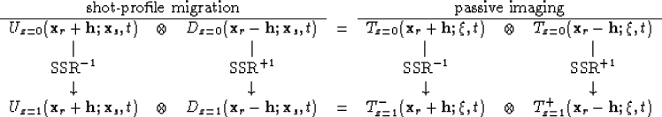
Figure ![[*]](http://sepwww.stanford.edu/latex2html/cross_ref_motif.gif) pictorially demonstrates how direct migration of
field passive seismic data fits into the framework of shot-profile
migration to produce the 0th and 1st depth levels of
the zero offset image. The sum over frequency has been omitted to
reduce complexity in the figure. Also, after the first extrapolation
step, with the two different phase-shift operators, the two
transmission wavefields are no longer identical, and can be redefined
U and D. This is noted with superscripts on the T wavefields at depth.
pictorially demonstrates how direct migration of
field passive seismic data fits into the framework of shot-profile
migration to produce the 0th and 1st depth levels of
the zero offset image. The sum over frequency has been omitted to
reduce complexity in the figure. Also, after the first extrapolation
step, with the two different phase-shift operators, the two
transmission wavefields are no longer identical, and can be redefined
U and D. This is noted with superscripts on the T wavefields at depth.
 |
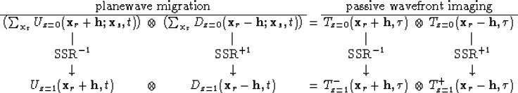
Shot-profile migration becomes
planewave migration if conventional shot-gathers are summed for wavefield
U, and a horizontal plane source is modeled for wavefield D. Partial
summation of conventional shot-records will introduce cross-talk
into the image. Only by summing enough shots so that their destructive
interference cancels out their cross-talk can one produce a high quality
image. For raw passive data, the sum over sources leads to an areal
wave with complicated temporal topography. Moving the sum over shots
in the imaging condition of equation 9 to operate on the
wavefields rather than their correlation, changes shot-profile
migration to something akin to planewave migration which I will call
wavefront migration.![[*]](http://sepwww.stanford.edu/latex2html/foot_motif.gif) Like planewave
migration, after even a few wavefields have been combined, the best
course of action is to sum all the sources to attain good areal
coverage of the source wavefront to minimize
cross-talk. Figure shows the change source
summation has on both conventional shot migration and direct passive
migration. Notice the parameterization of
Like planewave
migration, after even a few wavefields have been combined, the best
course of action is to sum all the sources to attain good areal
coverage of the source wavefront to minimize
cross-talk. Figure shows the change source
summation has on both conventional shot migration and direct passive
migration. Notice the parameterization of ![]() meaning field
data (where the depth subscript displaces the use of
Tf). Importantly, the data input into the migration needs to have
the late lags windowed before input into the migration as they have no
correspondence to the subsurface structure. This can be accomplished
by any of the three options discussed above: correlation followed by
windowing, DFT followed by subsampling, or stack followed by DFT and
correlation.
meaning field
data (where the depth subscript displaces the use of
Tf). Importantly, the data input into the migration needs to have
the late lags windowed before input into the migration as they have no
correspondence to the subsurface structure. This can be accomplished
by any of the three options discussed above: correlation followed by
windowing, DFT followed by subsampling, or stack followed by DFT and
correlation.
 |