


Next: Comparisons of conductivity bounds
Up: CONDUCTIVITY: CANONICAL FUNCTIONS AND
Previous: Estimation schemes based on
For random polycrystals (see the earlier discussion of the basic
model in the second section), it is most convenient to define a new
canonical function:
| ![\begin{displaymath}
\Sigma_X(s) = \left[\frac{1}{3}\left(\frac{1}{\sigma_H+2s}
+ \frac{2}{\sigma_M+2s}\right)\right]^{-1} - 2s,
\end{displaymath}](img116.gif) |
(36) |
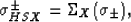
where the mean 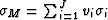 and harmonic mean
![$\sigma_H = \left[\sum_{i=1}^J \frac{v_i}{\sigma_i}\right]^{-1}$](img118.gif) of the layer constituents are the pertinent conductivities (off-axis
and on-axis of symmetry, respectively) in each layered grain. Then, the
Hashin-Shtrikman bounds for the conductivity of the random polycrystal are
of the layer constituents are the pertinent conductivities (off-axis
and on-axis of symmetry, respectively) in each layered grain. Then, the
Hashin-Shtrikman bounds for the conductivity of the random polycrystal are
|  |
(37) |
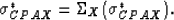
where  and
and  .These bounds are known not to be the most general ones since they rely
on an implicit assumption that the grains are equiaxed.
A more general lower bound that is known to be optimal is due to Schulgasser
(1983) and Avellaneda et al. (1988):
.These bounds are known not to be the most general ones since they rely
on an implicit assumption that the grains are equiaxed.
A more general lower bound that is known to be optimal is due to Schulgasser
(1983) and Avellaneda et al. (1988):
|  |
(38) |
Helsing and Helte (1991) have reviewed the state of the art for
conductivity bounds for polycrystals, and in particular have noted
that the self-consistent
[or CPA (i.e., coherent potential approximation)]
for the random polycrystal conductivity is given by
|  |
(39) |
It is easy to show (39) always lies between the two rigorous bounds
 and
and  , and also between
 and . Note that and cross when
  , with
becoming the superior lower bound for mean/harmonic-mean
contrast ratios greater than 10.
, with
becoming the superior lower bound for mean/harmonic-mean
contrast ratios greater than 10.
Next: Comparisons of conductivity bounds
Up: CONDUCTIVITY: CANONICAL FUNCTIONS AND
Previous: Estimation schemes based on
Stanford Exploration Project
5/3/2005