


Next: Implementation
Up: R. Clapp: Regularization
Previous: R. Clapp: Regularization
To map the irregular recorded seismic data onto the regular mesh
is a far from trivial.
A common approach in industry is to think of the problems in the same
way we approach Kirchhoff migration,
namely to loop over data space and spread into our regular
model space. The spreading operation can be governed by something
like AMO Biondi et al. (1998), which maps data from one offset vector to
another.
If we think of the AMO operator  as mapping from the regular model space
  to the irregular data space
  , our estimation procedure becomes,
|  |
(1) |
The wavenumber domain AMO operator works on a regular
sampled cube, so the problem is more complicated.
We first must map the data to a regular sampled space
by applying the interpolation operator  .The regular sampled cube
  is now a full five
dimensional volume (
is now a full five
dimensional volume (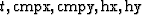 ).
We can produce the model at a given (hx,hy)
by summing nearby cubes (t, cmpx, cmpy) that have
transformed to our desired (hx,hy) through AMO.
To write this in a mathematical form we need
to make some definitions.
We will define ihx and ihy as the offset
indicies of the expanded space .These indicies correspond to the half-offset
hx and hy. The output space, , is defined
as a coralary ihx' and ihy` which also correspond
to hx and hy. The notation
).
We can produce the model at a given (hx,hy)
by summing nearby cubes (t, cmpx, cmpy) that have
transformed to our desired (hx,hy) through AMO.
To write this in a mathematical form we need
to make some definitions.
We will define ihx and ihy as the offset
indicies of the expanded space .These indicies correspond to the half-offset
hx and hy. The output space, , is defined
as a coralary ihx' and ihy` which also correspond
to hx and hy. The notation  correspond
to the 3-D subcube (t,cmpx,cmpy) at the given ihx' and
ihy'.
Finally
correspond
to the 3-D subcube (t,cmpx,cmpy) at the given ihx' and
ihy'.
Finally
 refers to
transforming the cube through AMO from the offset vector
refers to
transforming the cube through AMO from the offset vector  to
to  , nx and ny is the region in
sampling of that we wish to sum over; and
, nx and ny is the region in
sampling of that we wish to sum over; and
 and
and  is the sampling of
the cube in
is the sampling of
the cube in  and
and  respectively.
We obtain
respectively.
We obtain
|  |
(2) |
In we to write our regularization problem in the form of
equation (2),  is a
spraying operation
where the columns of the matrix are defined
by equation (1).
We then obtain or model by applying
is a
spraying operation
where the columns of the matrix are defined
by equation (1).
We then obtain or model by applying
|  |
(3) |
The formulation suffers from all of the usual problems associated with
applying an adjoint operation. We are spraying into a regular mesh, but
the data is not regular. Areas with higher
concentration of data traces will tend to map to artificially higher amplitudes in the model
space.
In the Kirchoff formulation
we can do some division by hit count to help minimize this effect.
Because we are operating in the wave number domain
we can't normalize by something as simple as hit count.
We can accomplish something similar by
following the approach of Claerbout and Nichols (1994) and Rickett (2001).
We approximate the Hessian of the least squares solution,
| 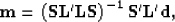 |
(4) |
by the diagonal operator  .We form by
| ![\begin{displaymath}
{\bf W^{-1}} = {\rm diag} \left[ \left( \bf S' \bf L' \bf L\bf S {\bf 1} +\alpha \right)\right]
,\end{displaymath}](img21.gif) |
(5) |
where  is a vector of 1s,
  is a stabilization term,
and
is a stabilization term,
and ![${\rm diag}[]$](img24.gif) map the vector to the diagonal of the matrix.
We scale our adjoint solution by obtaining
map the vector to the diagonal of the matrix.
We scale our adjoint solution by obtaining
| 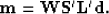 |
(6) |