Computing derivatives on a semistructured mesh

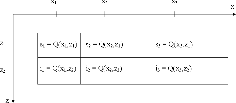
Let $Q(\omega, x, z)$ denote a 2D zero-offset seismic wavefield, regularly sampled (and Fourier transformed) in time, but irregularly sampled in space. The measured surface dataset is $Q(\omega, x, z=0)$. For downward continuing Q with (1) we need to write differencing stars for $\frac{{\partial Q}}{{\partial z}}$ and for $\frac{{\partial^2 Q}}{{\partial x^2}}$. Fig. 1 shows the differencing star for the entire equation and defines shorthand notations.

 

diffstar Figure 1 Differencing star for solving eq. 1 with the finite difference method; s1, s2, s3, i1, i2, i3 are just notations. This is the general case: the distance x2 - x1 is not necessarily equal to x3 - x2.

Since the differencing star spans only two values of z, it does not matter whether the sampling along the z axis is regular or not. I denote:  

$$z_2 - z_1 = \delta z.$$ (2)

All derivatives will be considered to be computed in the middle of the differencing star. When x₂ - x₁ = x₃ - x₂, the middle is in x₂. When the two distances are drastically different, the middle is not in x₂ any more and errors are introduced. This may be the cause of the spurious reflections off the large variations in grid steps that are visible in the bottom panel of Fig. 4. Dellinger and Muir (1986) discuss this problem and suggest that letting the gridpoints drift across x as we downward continue can solve it. In order to examine the extent to which this problem affects the data, I will simply pretend that the problem does not exist, and observe its negative effects. So, given the values of a function y(x) in three points, x₁, x₂ and x₃, with x₁ < x₂ < x₃, the second derivative can be computed by finding the coefficients of parabola that fits through the three points. The second derivative is twice the coefficient of the second-degree term in the parabola expression. Thus, by denoting:  

$$k_i = \frac{1}{{\prod\limits_{j \in \Psi - \left\{ i \right\}} {(x_j - x_i )} }},\quad i \in \Psi = \left\{ {1,2,3} \right\},$$ (3)

which can be more explicitly written out as  

$$k_1 = \frac{1}{{(x_3 - x_1 )(x_2 - x_1 )}},$$ (4)

 

$$k_2 = \frac{-1}{{(x_3 - x_2 )(x_2 - x_1 )}},$$ (5)

 

$$k_3 = \frac{1}{{(x_3 - x_1 )(x_3 - x_2 )}},$$ (6)

the second derivative is

 

$$\frac{{d^2 y}}{{dx^2 }} = 2\left( k_1 y_1 + k_2 y_2 + k_3 y_3 \right).$$ (7)

The same formula is obtained by computing a first-order approximation of the second derivative as the first derivative of the first derivative in the point x₂. It should be noticed that the Laplacian is a low-pass filter of the original functionr. In other words, the curvature of the hyperbola is the same in each of the three points it fits through; x₃ - x₂ must be really different from x₂ - x₁ in order for the curvature-fitting hyperbola to be affected by the error and for artifacts to be generated. This explains why the method is so robust. As Fig. 3 shows, artifacts start to become barely visible when x₃ - x₂ = 2(x₂ - x₁). The partial derivatives in x of even order higher than two of the wavefield will be even more robust. A method that would make use not of the second-order derivatives but of the fourth-order ones, would be much less affected by the spurious reflections.

Using the notations in Fig. 1 and eq. (2), the second derivative expression in (7), and employing a Crank-Nicolson scheme to compute the second derivative in x, we obtain the following differencing stars:

 

$$\frac{{\partial^2 Q}}{{\partial x^2}} = k_1(i_1 + s_1) + k_2(i_2 + s_2) + k_3(i_3 + s_3),$$ (8)

 

$$\frac{{\partial Q}}{{\partial z}} = \frac{1}{\delta z}(i_2 - s_2),$$ (9)

 

$$\frac{{\partial^3 Q}}{{\partial z\partial x^2}} = \frac{2k_1... ...{2k_2}{\delta z}(i_2 - s_2) + \frac{2k_3}{\delta z}(i_3 - s_3).$$ (10)

The way the derivatives of a function are computed on a irregular mesh does not depend on the nature of the function, but the result of the computation does: the lower the frequency content, the better. This means that longer wavelengths will generate less artifacts, and the spatio-temporal frequency content of the spurious reflections will therefore be biased towards the high part of the spectrum. Practically no artifacts should be produced when the function has a very low frequency content, as is the case with potential fields. Upward or downward continuation of potential fields on a unstructured mesh should be very accurate.