Regularization after binning: missing data interpolation

One of the factors affecting the convergence of iterative data regularization is clustering of data points in the output bins. Since least-squares optimization assigns equal weight to each data point, it may apply inadequate effort to fit a cluster of data points with similar values in a particular output bin. To avoid this problem, we can replace the regularized optimization with a less accurate but more efficient two-step approach: data binning followed by missing data interpolation.

Missing data interpolation is a particular case of data regularization, where the input data are already given on a regular grid, and we need to reconstruct only the missing values in empty bins. Claerbout (1992) formulates the basic principle of missing data interpolation as follows:

A method for restoring missing data is to ensure that the restored data, after specified filtering, has minimum energy.

Mathematically, this principle can be expressed by the simple equation  

$$\bold{D m \approx 0}\;,$$ (73)

where $\bold{m}$ is the data vector and $\bold{D}$ is the specified filter. Equation () is completely equivalent to equation (). The approximate equality sign means that equation () is solved by minimizing the squared norm (the power) of its left side. Additionally, the known data values must be preserved in the optimization scheme. Introducing the mask operator $\bold{K}$, which can be considered as a diagonal matrix with zeros at the missing data locations and ones elsewhere, we can rewrite equation () in the extended form  

$$\bold{D (I-K) m} \approx - \bold{D K m} = - \bold{D m}_k\;,$$ (74)

in which $\bold{I}$ is the identity operator, and $\bold{m}_k$represents the known portion of the data. It is important to note that equation () corresponds to the limiting case of the regularized linear system  

$$\left\{\begin{array} {l} \bold{K m} = \bold{m}_k\;, \\ \epsilon \bold{D m} \approx \bold{0}\end{array}\right.$$ (75)

for the scaling coefficient $\epsilon$ approaching zero. System () is equivalent to system (-) with the masking operator $\bold{K}$ playing the role of the forward interpolation operator $\bold{L}$. Setting $\epsilon$ to zero implies putting far more weight on the first equation in () and using the second equation only to constrain the null space of the solution. Applying the general theory of data-space regularization from Chapter , we can immediately transform system () to the equation  

$$\bold{K P p} \approx \bold{m}_k\;,$$ (76)

where $\bold{P}$ is a preconditioning operator, and $\bold{p}$ is the preconditioning variable, connected with $\bold{m}$ by the simple relationship

$$\bold{m} = \bold{P p}\;.$$

According to equations () and () from Chapter , equations () and () have exactly the same solutions if the following condition is satisfied:  

$$\bold{P}\,\bold{P}^T = \left(\bold{D}^T\,\bold{D}\right)^{-1}\;,$$ (77)

where we need to assume the self-adjoint operator $\bold{D}^T\,\bold{D}$ to be invertible. If $\bold{D}$ is represented by a discrete convolution, the natural choice for $\bold{P}$ is the corresponding deconvolution (inverse recursive filtering) operator:  

$$\bold{P} = \bold{D}^{-1}\;.$$ (78)

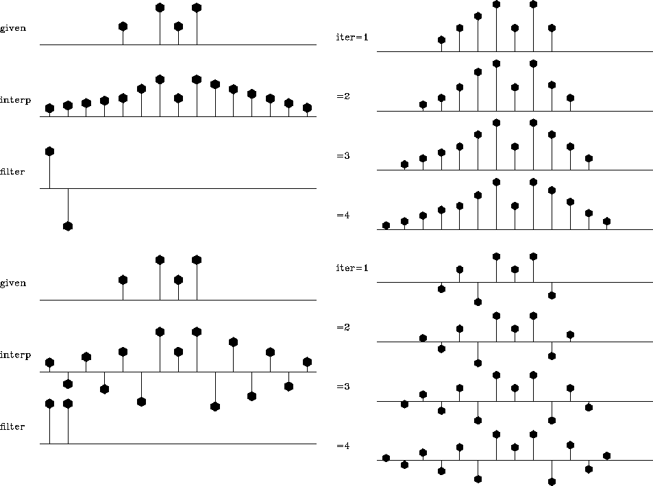
I illustrate the missing data problem with a simple 1-D synthetic data test taken from Claerbout (1999). Figure  shows the interpolation results of the unpreconditioned technique with three different filters. For comparison with the preconditioned scheme, I changed the boundary convolution conditions from internal to truncated transient convolution. As in the previous example, the system was solved with a conjugate-gradient iterative optimization.

 

mall
Figure 8 Unpreconditioned interpolation with two different regularization filters. Left plot: the top shows the input data; the middle, the result of interpolation; the bottom, the filter. The right plot shows the convergence process for the first four iterations.

As depicted on the right side of the figures, the interpolation process starts with a ``complicated'' model and slowly ``simplifies'' it until the final result is achieved.

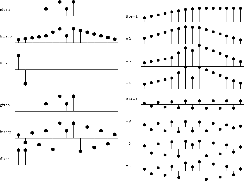
Preconditioned interpolation (Figure ) behaves differently. At the early iterations, the model is simple. As the iteration proceeds, new details are added into the model. After a surprisingly small number of iterations, the output closely resembles the final output. The final output of interpolation with recursive deconvolution preconditioning is exactly the same as that of the original method.

 

sall
Figure 9 Interpolation with preconditioning. Left plot: the top shows the input data; the middle, the result of interpolation; the bottom, the filter. The right plot shows the convergence process for the first four iterations.

The next section extends the idea of preconditioning by inverse recursive filtering to multiple dimensions.