 |
||
| (7) |
 |
Starting from the eikonal equation in the time coordinates,
we can remap the tomography goals of equation (6)
into the time coordinates.
The operators ![]() ,
, ![]() ,
, ![]() are different in the time domain from the equivalent
depth-domain operators;
and also
are different in the time domain from the equivalent
depth-domain operators;
and also ![]() has a slightly different orientation,
because it now operates on a velocity function defined in (
has a slightly different orientation,
because it now operates on a velocity function defined in (![]() ,
,![]() ).
).
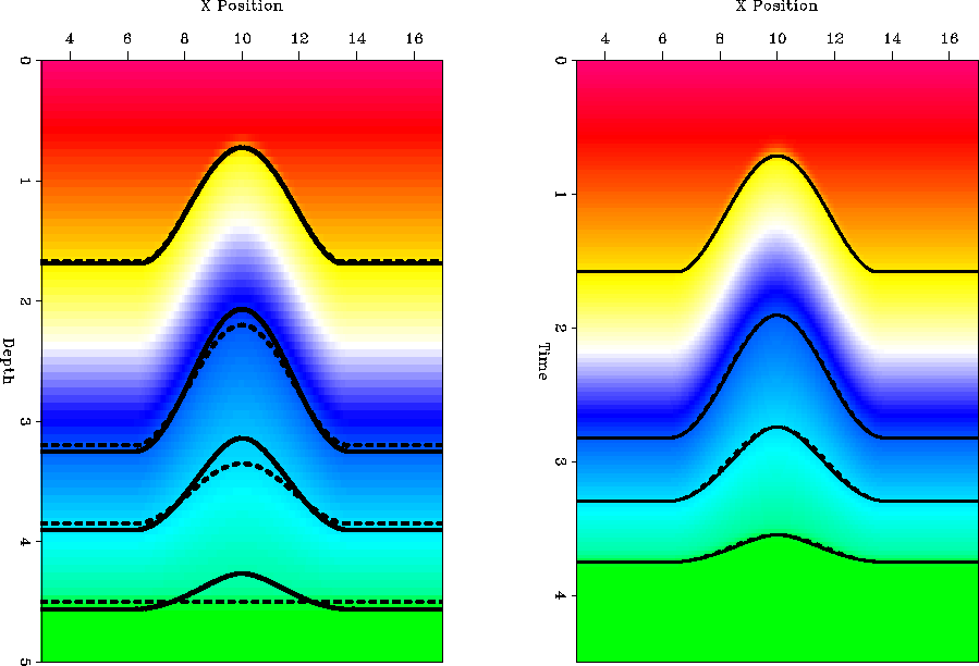
Some of the advantages of
formulating the tomography problem in (![]() ,
,![]() ) domain
can be seen in Figure 9.
In this new domain reflector
movement is minimal,
significantly decreasing the velocity-depth connectivity problem that
we saw in (z,x) space.
The initial reflector position is closer to
the correct reflector position.
As a result, the orientation of the steering filters
more accurately follows true reflector dip.
) domain
can be seen in Figure 9.
In this new domain reflector
movement is minimal,
significantly decreasing the velocity-depth connectivity problem that
we saw in (z,x) space.
The initial reflector position is closer to
the correct reflector position.
As a result, the orientation of the steering filters
more accurately follows true reflector dip.
 |
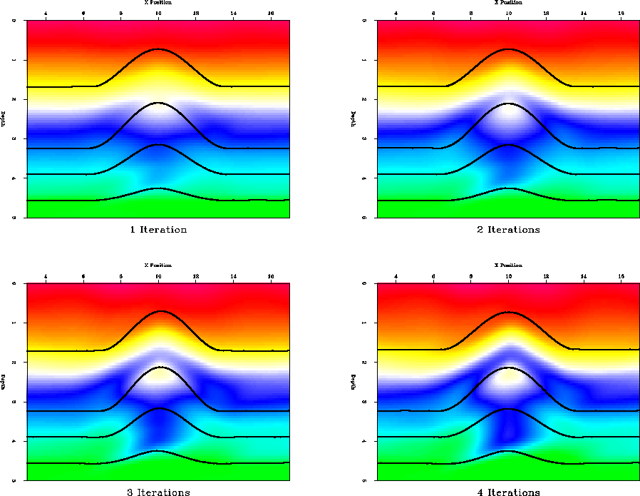
To analyze the advantages of working in (![]() ,
,![]() ) space we performed
two non-linear iterations of tomography and remapped the resulting
velocity model back into (z,x) space (Figure 10).
Comparing the results of tomography in the time domain
(Figure 10),
with the results of tomography in the depth domain
(Figure 8),
we can notice how the doublet,
seen in the depth tomography case, has significantly
decreased and how the dome shape is much more prominent.
) space we performed
two non-linear iterations of tomography and remapped the resulting
velocity model back into (z,x) space (Figure 10).
Comparing the results of tomography in the time domain
(Figure 10),
with the results of tomography in the depth domain
(Figure 8),
we can notice how the doublet,
seen in the depth tomography case, has significantly
decreased and how the dome shape is much more prominent.