Next: Synthetic Example
Up: Clapp & Biondi: Velocity
Previous: INTRODUCTION
We can write our fitting goals for a linear problem as
|  |
(1) |
Where  is the data,
  is the linearized tomographic operator, and
 is our model.
Often the problem is under-determined,
so we need to add some type of regularization
is our model.
Often the problem is under-determined,
so we need to add some type of regularization
|  |
(2) |
Ideally,  should be the inverse of the model covariance matrix
Tarantola (1987).
Unfortunately, we are
estimating the model so we don't have the covariance matrix.
The lack of knowledge about the model often leads to the Laplacian
or some other isotropic
operator being used for .
As a result, we fill the null-space of the model with isotropic features, that,
while explaining the data,
may be unreasonable when judging the results
with geologic criteria.
should be the inverse of the model covariance matrix
Tarantola (1987).
Unfortunately, we are
estimating the model so we don't have the covariance matrix.
The lack of knowledge about the model often leads to the Laplacian
or some other isotropic
operator being used for .
As a result, we fill the null-space of the model with isotropic features, that,
while explaining the data,
may be unreasonable when judging the results
with geologic criteria.
Fortunately, we often do have other sources of information, such as a
geologist's model for the region or reflector dip from
well logs, that can be used to better constrain our
inversion.
For example, we can the find the general dip
direction by interpreting an early migration result
and use this information to construct a space variant filtering operator
that annihilates dips with the given direction.
(Figure 1),
that can be used as in equation (2).
The inverse of the dip-annihilation operator
is really a first-order approximation
for the model covariance matrix.
We know that in general we have some isotropic smoothness
in our velocity function, therefore
adding some isotropic smoothness to our regularization
operator is appropriate.
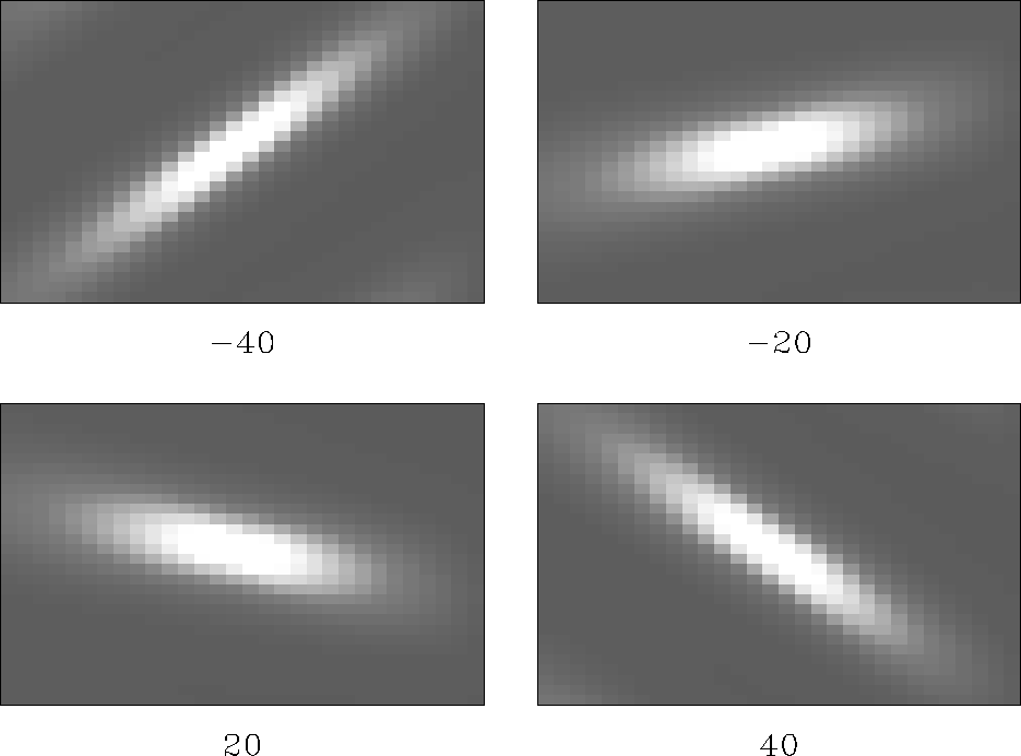
This creates
a space variant filter
direction and produces an anisotropic blob oriented in the dip direction
(Figure 2).
filters
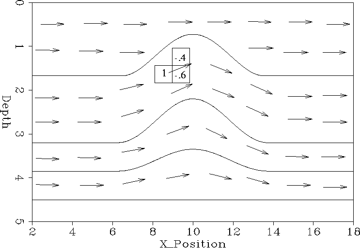
Figure 1 Steering filter directions as a function of
geologic dip.
 sweep
sweep
Figure 2 Preconditioning operator impulse response when oriented at -40, -20, 20, and 40 degrees from horizontal.


By forming our operators in helix-space Claerbout
1997,
we can find a stable inverse for our
steering filters () and change our regularization problem into a preconditioning problem.
By substituting:
|  |
(3) |
we get
|  |
|
| (4) |
The inverse operator ( ) spreads information long distances
at every iteration, quickly filling the null-space with reasonable values.
) spreads information long distances
at every iteration, quickly filling the null-space with reasonable values.
In general,
tomography problems are not as straightforward as the one presented
above. First and foremost, the tomography problem is non-linear.
Perturbations in the slowness model change the raypaths,
making the tomography problem non-linear.
We can get around this by imposing an outer, non-linear raytracing loop
over a linearized back projection operation that assumes stationary
raypaths.
In addition, we must deal
with the inherent velocity-depth coupling problem: any changes
in traveltimes can be caused by either reflector movement or slowness
model changes.
Therefore, we must take into account reflector movements
when evaluating the linearized tomographic operator van Trier (1990):
|  |
(5) |
where

- is the difference between the modeled
and the correct travel times,

- is the back-projection operator along our modeled
ray paths,

- maps changes in reflector position to changes in traveltimes,

- is the change in reflector position,

- maps slowness changes to reflector movement,

- is -ur change in slowness.
Finally, we add in our preconditioning operator
to obtain our final set of tomography goals,
|  |
|
| (6) |
Next: Synthetic Example
Up: Clapp & Biondi: Velocity
Previous: INTRODUCTION
Stanford Exploration Project
7/5/1998