 |
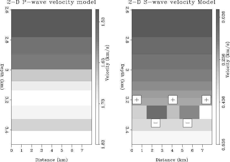
Figure 8 P-wave and S-wave interval velocity models.
In this section, I explore the effect of a full 2-D inversion for P- and S-impedance contrasts as opposed to the local observation of AVO amplitudes. I constructed a 2-D model consisting of the blocked sonic velocities and densities. They were kept laterally constant. The S-wave velocity model does have laterally changing S-wave velocities across the BSR. These variations have the same magnitudes as in the previous section. The sonic and shear velocities are displayed in Figure 8.
 |
After generating CMP gathers every 50 m along the 2-D model, I performed a true amplitude migration in order to collapse the diffractions caused by the laterally varying S-wave velocity contrasts. Subsequently, I applied a least-squares impedance inversion Lumley and Beydoun (1993). This technique fits the prestack migrated AVO gathers at each pseudo-depth and surface position to the theoretical P- and S-impedance curves based on the linearized Zoeppritz equations. The study was performed both for noise free and noisy data.
Figure 9 shows the noise free P- and S-impedance contrast sections zoomed in around the BSR. It shows a strong negative P-impedance contrast (black), and the variations from positive to negative S-wave impedance contrasts. The result based on noisy data is shown in Figure 10. The signal to noise ratio was again approximately 2:1 for the BSR amplitudes. As expected, the P-wave impedance looks very similar to the previous one. The S-wave impedance, on the other hand, appears much noisier than before. It is harder to differentiate between the small positive and negative contrasts between 4 and 6 km distance. Since the P-impedance contrast is uniform through the section, a P*S impedance map should emphasize areas where the P-and S-impedance are either both negative/positive or have different sign. This will give some insight into the qualitative behavior of the shear wave velocity from hydrate to the underlaying sediments. The result can be seen in Figure 11.
Although the data is contaminated by noise, the P*S impedance contrast map shows the areas of negative S-wave velocity contrasts (white) and positive S-wave velocity contrast (black). Even the small contrasts are visible in the map. Though the amplitudes of the data can not be distinguished using a 1-D local AVO analysis, the 2-D inversion and subsequent properly chosen attribute map results in a higher resolution. When picking the amplitudes along a reflector, one usually picks the maximum positive or negative peaks. These may, however, not always line up perfectly after NMO correction. Thus, when fitting the theoretical impedance curves to each pseudo-depth surface position, which is done along a straight line, the 2-D inversion already somewhat averages out some of the noise.