 |
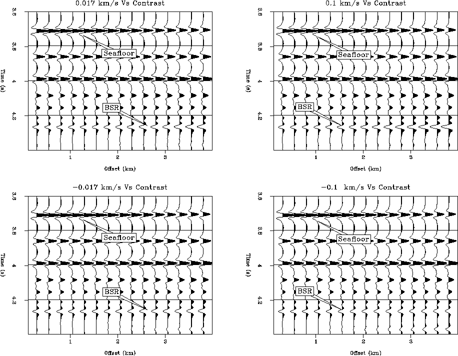
Figure 2 S-wave velocity contrast variations across the BSR. The left panels shows an increase in the shear contrast (+), while the right one shows a decrease in shear contrast (-). The contrasts vary from
The blocked data described in the previous section are used to evaluate the effect of different shear velocity contrasts across the BSR on seismic amplitudes. To do so, I vary the contrast at the transition from hydrate bearing sediments to the underlying gas sediments. In this way, I simulate either a positive shear wave velocity contrast or a negative shear wave velocity contrast (Figure 2). A positive contrast is characterized by an increase of the shear wave velocity at the transition from hydrate to gas, while a negative contrast means that Vs decreases across the BSR.
 |
The forward modeling was performed by generating synthetic seismograms using a generalized Kirchhoff body force scattering theory by Lumley and Beydoun Lumley and Beydoun (1993). This technique combines Zoeppritz plane-wave reflection and Rayleigh-Sommerfeld elastic diffraction responses and generates correct AVO responses for locally planar reflectors. The method computes only primary reflections, which is, however, sufficient for this case. Due to the very thick water layer of nearly 3 km, seismic data do not show multiple contamination or converted shear waves. I used the blocked elastic parameters described before as input into the modeling code and generated CMP gathers with different shear contrasts across the BSR. The P-wave velocities and densities were kept constant. Each CMP gather has a near-offset of 0.3 km and a far offset of 3.9 km. The offset spacing is 50m. This simulates the typical surface seismic aquisition scheme used to acquire data in the Blake Ridge region.
 |
Figure 3 shows the modeling result after applying spherical
divergence correction and NMO correction. The upper two CMP gathers
were obtained by assuming a positive shear contrast at the BSR, the
lower ones were generated with a negative contrast. The contrasts varied
from being very small (![]() 17 m/s) to being about
17 m/s) to being about ![]() 100 m/s.
The synthetic gathers
show that the positive contrast is characterized by an increase in the
BSR amplitude with increasing offset. The negative contrasts display the
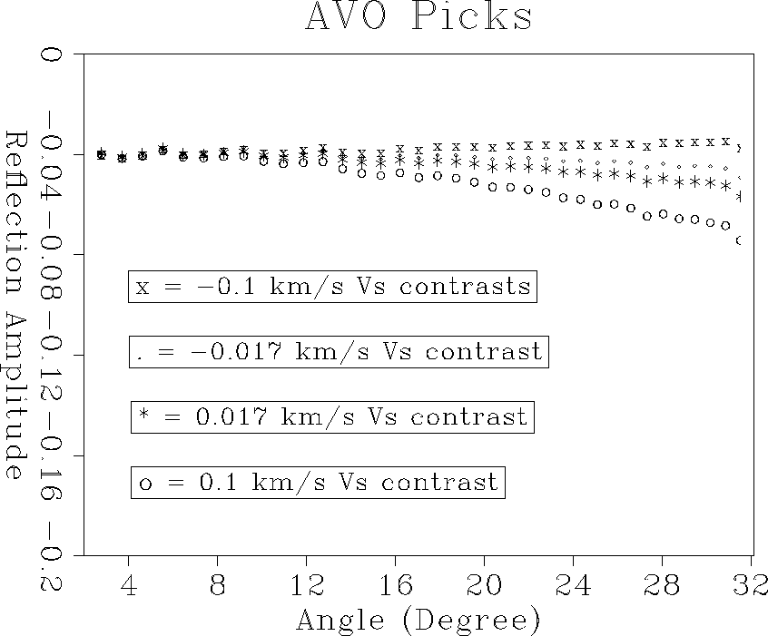
reverse behavior. To emphasize the different amplitude behavior, I picked the
amplitudes in each CMP gather along the BSR reflection at approximately
4.29s two-way traveltime. The picked amplitudes can be seen in
Figure 4.
100 m/s.
The synthetic gathers
show that the positive contrast is characterized by an increase in the
BSR amplitude with increasing offset. The negative contrasts display the
reverse behavior. To emphasize the different amplitude behavior, I picked the
amplitudes in each CMP gather along the BSR reflection at approximately
4.29s two-way traveltime. The picked amplitudes can be seen in
Figure 4.
 |
The picked AVO curves can be uniquely distinguished at large angles even in case of very small shear contrasts. Since the P-wave velocities and densities did not change during the modeling, the curves are in agreement for small angles. They start to differ at larger angles due to the changing shear wave velocity contrasts. Least-squares inversion using the linearized Zoeppritz equation will result in well constrained P- and S-impedance contrasts.
Real data, on the other hand, never display such a clean amplitude behavior. Amplitudes are affected by different phenomena such as transmission, array attenuation, spherical divergence, multiples, random noise and so on. Processing to recover the true amplitude unperturbed by those effects has the danger of not correcting for all occurring amplitude losses or not preserving the amplitude information. This will lead to errors in the amplitudes that can not be easily quantified anymore. In the case of ideal processing and correcting, the data will still be contaminated by random noise which will influence the amplitudes.
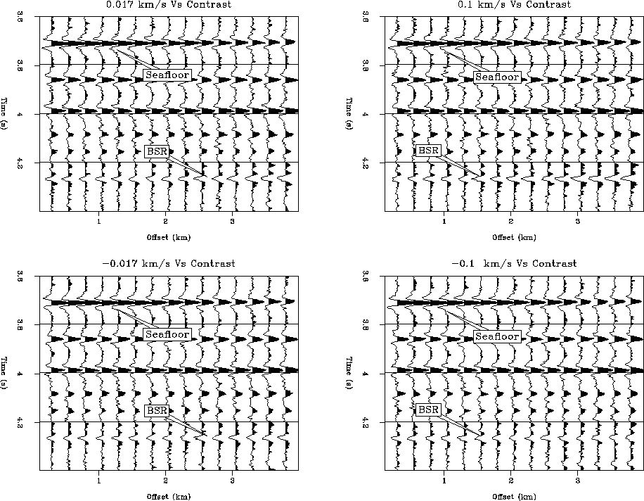
In order to simulate a more realistic data setting, I added random Gaussian noise to my data. The magnitude of the noise was approximately half that of the near offset BSR amplitude. The resulting noisy CMP gathers can be seen in Figure 5. The data display quite a variance in their amplitudes and obvious distortions.
 |
For the detection of the elastic layer properties from the BSR AVO behavior, it is important to know how long these amplitudes can still be uniquely distinguished using AVO analysis. This concerns the far offsets in particular since they carry all the S-wave velocity information. Using the known standard deviation of the data, it is possible to put error bars around the noise free amplitude and predict the variance of the noisy data and thus the possible resolution of two different AVO events. Figure 6 shows the true amplitude picks for data with the corresponding error bars. The error bars give a 95% confidence interval for the deviation of the noisy data from the true data at a certain angle. Amplitude picks from two different CMP gathers can only be resolved in their curvature when the difference between the true values is larger than the error bar. Since the AVO curves will agree at small angles due to the same P-wave velocity and density contrast, Figure 6 focuses on angles above 25 degrees.
The left panel of figure 6 shows the comparison of amplitudes
associated with ![]() 17 m/s shear contrast across the BSR. It is obvious that
these two events will not be resolvable once the noise is added to
the data. The middle panel shows a comparison between amplitudes caused by
17 m/s shear contrast across the BSR. It is obvious that
these two events will not be resolvable once the noise is added to
the data. The middle panel shows a comparison between amplitudes caused by
![]() 50 m/s Vs-contrasts. In this case, the two events might barely be
distinguished. For
50 m/s Vs-contrasts. In this case, the two events might barely be
distinguished. For ![]() 100 m/s contrasts, however, there appears to be
a clear resolution between the data at large angles.
100 m/s contrasts, however, there appears to be
a clear resolution between the data at large angles.
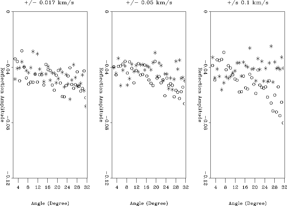
Figure 7 displays the actual picked BSR amplitudes from
the synthetic, noisy CMP gathers. As predicted from the error bars, the picks
from ![]() 17 m/s Vs-contrasts cannot be distinguished anymore. The data also shows
a lot of overlapping for the case of
17 m/s Vs-contrasts cannot be distinguished anymore. The data also shows
a lot of overlapping for the case of ![]() 50 m/s shear velocity contrasts.
However, as the prediction has shown, these might be just resolvable. It is
obvious, however, that the picks of the 100 m/s and -100 m/s contrasts are
distinguishable.
50 m/s shear velocity contrasts.
However, as the prediction has shown, these might be just resolvable. It is
obvious, however, that the picks of the 100 m/s and -100 m/s contrasts are
distinguishable.
In the case of a least-squares inversion of these data
for the layer properties,
this means that there would be at least an error of ![]() 50 m/s on an
observed shear contrast, if not more. In the case of small contrasts,
even the sign of the S-wave velocity contrast (positive or negative) cannot be
uniquely inferred anymore. The error will of course vary with the amount of
deviation in the amplitude. As mentioned before, the P-wave velocity
contrast is
much more stable even for such data variance and will be better constrained.
50 m/s on an
observed shear contrast, if not more. In the case of small contrasts,
even the sign of the S-wave velocity contrast (positive or negative) cannot be
uniquely inferred anymore. The error will of course vary with the amount of
deviation in the amplitude. As mentioned before, the P-wave velocity
contrast is
much more stable even for such data variance and will be better constrained.
In order to improve the data quality and to reduce the random noise, one could assume that the lateral layer properties do not change significantly over a certain region. In that case, the averaging of the amplitudes of several CMPs will give an improved AVO response. However, also in this case the small shear contrasts and thus the important uniqueness of the sign of the contrast might be lost.
 |
 |