Masking function

Transformation of CMP data to a space parameterized by (t,h,p) allows the predicted primary and first water bottom related multiple events to be represented by a simple smooth surface. This simple representation of the primary and multiple trends allows for a distinct separation of primary and multiple energy.

The mask we used to separate the multiple energy from the primary energy is a volume in the model space defined by two surfaces; one surface follows the trend of the predicted primary events and the other follows the trend of the predicted first water bottom related multiple events. The predicted trends are determined for offset and time values corresponding to each of the values of stepout evaluated by the beam stack inversion. In order to preserve the multiple energy alone, we retain the energy that resides at near offsets and later times relative to the multiple trend surface, and mute out the energy that resides at far offsets and earlier times relative to the primary trend surface. In the region between these two surfaces we use a linear weighting function. This weighting function is zero at the primary surface and unity at the multiple surface. Building a linear weighting between the predicted primary and multiple trend eliminates many of the effects due to truncation artifacts that would appear if a simple step function were used to separate the energy. Truncation artifacts are a significant problem associated with forward modeling of beam stacked data because events in beam stacked space have significant extent in the offset and stepout dimensions.

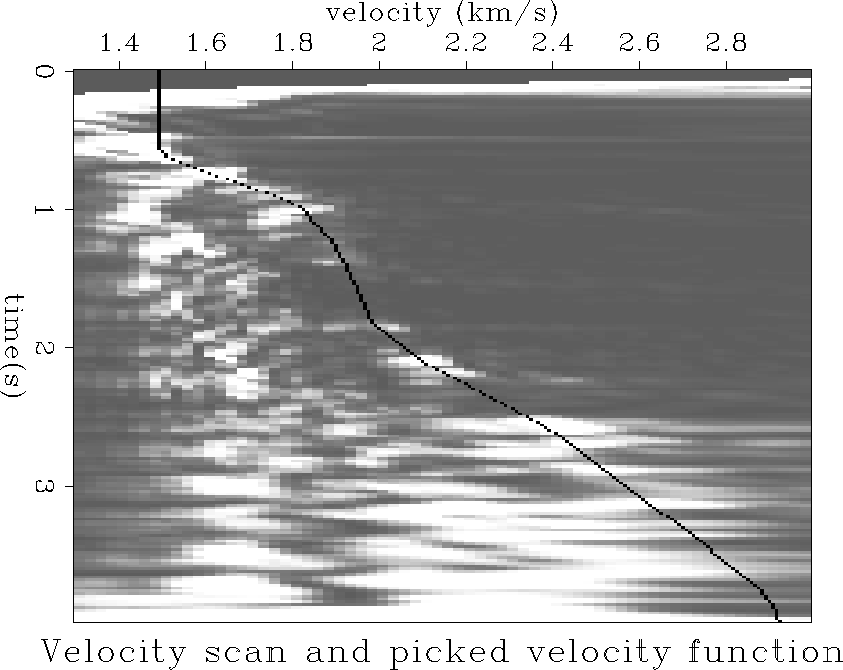
We obtained the primary velocity trend by manually picking a velocity scan of a gather 807 of the Mobil AVO dataset Figure 3.

 

velplot Figure 3 Velocity scan of the Mobil AVO data. The picked velocity function used in this paper is superimposed onto the scan.

With the velocity trend V(t₀) we predict for each stepout p:

• The expected offset of the primary trend h_p(t₀,p) for each value of t₀.
  
• The two way travel time t_p(t₀,h_p) of the primary trend corresponding to the offset h_p(t₀,p).

An analyitic relation between the offset of the primary trend as a function of t₀ is often not possible, because V_p(t) is usually obtained from a velocity scan. In order to construct the primary surface in the (t,h,p) space, we use the relations given below for the offset and two-way travel time of an event, and linear interpolate between the calculated points.

$$\begin{eqnarray} h_{p}(t_0,p) &=& \frac{pt_0V_{p}(t_0)^2}{\sqrt{1-(pV_{p}(t_0))^2}}\end{eqnarray}$$ (8)

$$\begin{eqnarray} t_{p}(t_0,h_p) &=& \sqrt{t_{0}^2+\frac{h_p^2}{4V_{p}(t_0)^2}}\end{eqnarray}$$ (9)

The second equation is simply the Dix equation for a hyperbolic event with velocity V_p(t₀), offset h_p and the zero offset travel time t₀. The first equation is derived from Dix equation, but with the time t_p being replaced by the following equation also derived from the Dix equation:

$$\begin{eqnarray} t\frac{dt}{dh} &=& \frac{h}{4V_{p}(t_0)^2} \\ t_{p}(h_p,p) &=& \frac{h}{4pV_{p}(t_0)^2} \end{eqnarray}$$ (10) (11)

This is the two way travel time to an event parameterized by velocity V(t₀), at the stepout p and offset h of that event. When this is substituted into the Dix equation the resulting equation for offset is given by equation (1). The above relations are strictly derived from the Dix equation and thus represent the offsets and travel times of the hyperbolic events with zero offset travel time t₀ and stepout p.

We estimate the velocity trend of the multiple energy from the RMS equation. In the following equation the primary velocity trend is V_p(t₀), the zero offset travel time to the water bottom is t_w, the travel time for each interval is $\Delta_i$ and v_w is the velocity of the water layer. Lumley et al. (1994).

$$\begin{eqnarray} V_m(t_0+t_w) &=& \frac{\sum v_i\Delta_i+t_{w}v_{w}^2}{t_{0}+t_w}\end{eqnarray}$$ (12)

A Taylor series expansion of the above equation about t_w to the second order gives:

$$\begin{eqnarray} V_m(t_0+t_w) &=& \frac{\sum v_i\Delta_i+t_{w}v_{w}^2}{t}(1-\frac{t_w}{t_{0}}+\frac{t_{w}^2}{t_{0}^2})\end{eqnarray}$$ (13)

$$\begin{eqnarray} V_m(t_0+t_w) &=& (V_{p}^2+\frac{t_{w}}{t}v_{w}^2)(1-\frac{t_w}{t_{0}}+\frac{t_{w}^2}{t_{0}^2})\end{eqnarray}$$ (14)

Thus the expressions for the multiple trend are:

$$\begin{eqnarray} h_m(t_0,p)&=& \frac{pt_0V_{m}(t_0)^2}{\sqrt{1-(pV_{m}(t_0))^2}}\end{eqnarray}$$ (15)

$$\begin{eqnarray} t_{m}(t_0,h_m) &=& \sqrt{t_{0}^2+\frac{h_p^2}{4V_{m}(t_0)^2}}\end{eqnarray}$$ (16)

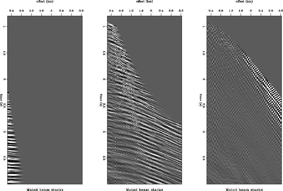
In beam stacked space the masking volume appears in each stepout panel as an area. The estimate of the multiple energy in beam stacked space is shown in Figure 4. The same three slowness slices of beam stacked space are shown in Figure 2 with out the muting applied.

 

cmp807m
Figure 4 Windowed multiples in beam stacked space; left p=0.03 (s/km), middle p=0.21(s/km) ,right p=0.69(s/km)

These figures illustrate the form of the muting function for three stepout slices of the (t,h,p) transformed cube. The energy at later times and near offsets relative to the muting function is preserved because this is exclusively multiple energy while the energy at earlier times and far offsets relative to the muting function have been zeroed because this is the region that exclusively contains primaries. The region between the primary surface and multiple surface is a region of overlap of the multiple and primary energy. An ideal transform to (t,h,p) space would put no energy in this region, but the events in beam stack space have significant extent in the offset direction. Using the linear weighting function gives the appropriate weight to the overlap energy in this region.

The left panel in Figure 4 corresponds to the first stepout value inverted for, 0.03 (s/km). The separation between primary and multiple energy in this panel is hard to discern because the moveouts of both primary and multiple events are nearly the same near zero offset. The second panel corresponds to a stepout value of 0.21 (s/km). In this image the train of multiples appear as a discernible trend which tracks linearly at an angle that lies at a stepout of about 2.67 (s/km). The primary trend has been muted out. The final image in the trio is the panel that corresponds to a stepout value of 0.69 (s/km). This is the velocity of the water column. Here it can be seen that only the water bottom energy at far offsets is stacked in while all the other locations in the gather contribute very little, as is expected.