


The synthetic subsurface image in Figure 3 simulates a delta with a slump fault. The model has horizontal layers near the top, a Gaussian appearance (the delta sediments) in the middle, and dipping layers on the bottom. Horizontal unconformities divide the three regions.
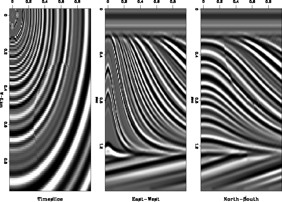 |
The left image of Figure 3 shows a horizontal time-slice from the middle of the model. A careful observer will notice the parabolic fault line in the center of the plot (Figure 4 displays the slump fault's location more visibly and may help locating it in Figure 3). The image in the center shows a vertical slice that corresponds to a cut in the North-South direction of the original model. (In general, we use by North-South and East-West to refer to the map-view as represented by the time-slice.) The cut is taken at the western edge of the model. Consequently, the section follows the gradient of the bedding and displays the maximal reflector dip of the model. The right image displays a vertical East-West slice that cuts the model at its center. The section intersects the slump fault The section's apparent bedding dip is smaller than the dip in the North-South section, since the center section is not parallel to the bedding's gradient.
Figure 4 displays the Lomoplan output corresponding to the time-slice in Figure 3. The top left plot shows the magnitude of the three Lomoplan output cubes. The other three plots are the individual Lomoplan residuals. Each panel is computed by 2-D prediction error filters operating in a different plane. The top right plot is generated by 2-D planar PE filters that operate in the time-slice plane, as the TS of the plot title indicates. The list a1=1, a2=7, a3=2 of the title expresses the filters' size: no extension in the depth dimension (thus a time-slice filter), seven samples in the North-South dimension, and two samples in the East-West dimension. The bottom right panel corresponds to vertical PE filters predicting in the East-West plane. Finally, the bottom left panel is the output of vertical 2-D PE filters in the North-South plane.
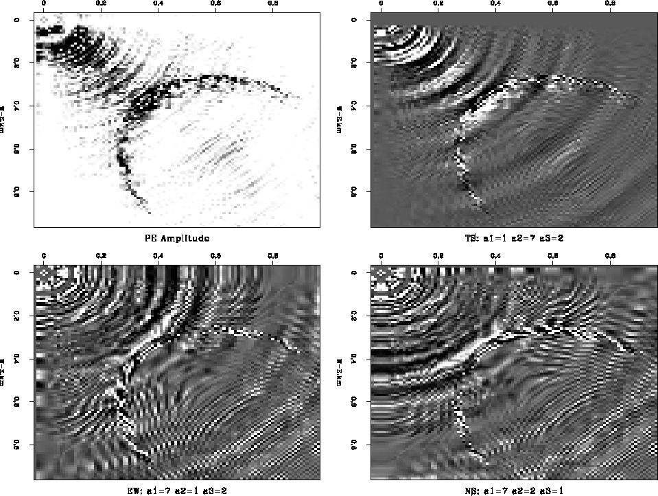 |
All three Lomoplan residuals in Figure 4 enhance the slump fault. The slump fault is characterized by relatively strong but random output values. All three panels display characteristic noise: the time-slice prediction could not predict the steeply dipping and strongly curving events close to the image's diagonal. At these locations, the synthetic model probably violates our assumption that the model can be locally represented as planar reflector model. The time-slice filter succeeded, however, in removing the same events where they were oriented parallel to one of the filter's axes, as at the northern and western edge of the image. This may indicate unfavorable directional bias that probably results from our filter shape. Both vertical filters display a ringing noise, which might be related to the interpolation that generated the synthetic image. The East-West filter perfectly rejects the East-West striking events at the western edge of the model, but it fails to reject the steeply North-South dipping events at the northern edge of the image. Contrarily, the North-South filter rejects the events at the northern edge, but fails at the western edge. This indicates that the filter with depth stepout of seven coefficients has not sufficed to remove the events of steep apparent dip.
We combined the three Lomoplan outputs by computing the L-2 norm amplitude of the three component vector residual (time-slice, East-West, North-South) at each location. The resulting amplitude at the left top corner of Figure 4 shows no image improvement over the individual residual plots. The time-slice residual dominates the amplitude plot, since its values are an order of magnitude larger than the values of the two vertical residuals. Since the amplitude plot adds positive numbers, the noise is not cancelled. This synthetic model demonstrates our need for a better method to combine the various residual images of Lomoplan.


