|
|
|
|
Identifying reservoir depletion patterns from production-induced deformations with applications to seismic imaging |
Although the asymptotic technique discussed in an earlier section addresses to some extent the issue of inhomogeneous models, it is inherently limited to moderate heterogeneity. However, practical applications of this method would require a more accurate handling of heterogeneity. Because layered models are of particularly high importance due to their commonality, we first consider modeling displacements for a vertically heterogeneous and horizontally slowly-varying medium. Rather than trying to solve a heterogeneous analogue of system 1 and 2, we will assume that one or all components of the displacement at a fixed depth
 immediately above the reservoir are known a priori. For example, we may use operator 5 to model displacements near the reservoir where the effect of the spatial heterogeneity of elastic parameters is limited. With displacements at
and free-surface boundary conditions at
immediately above the reservoir are known a priori. For example, we may use operator 5 to model displacements near the reservoir where the effect of the spatial heterogeneity of elastic parameters is limited. With displacements at
and free-surface boundary conditions at  , the problem of modeling subsurface displacements is reduced to solving a boundary-value problem for the elastostatic system:
 denote the stress tensor components, summation is carried out on repeating indices and body-force distribution is zero. The boundary conditions used with system 14 are the following:
 is a known displacement field at a fixed depth. Although system 14 is comprized of purely elastostatic equations, it allows us to model fluid-to-solid coupling via the boundary condition at
 that can be approximately computed using operator 5. For a laterally-homogeneous medium - or under the assumption of slow lateral variability and pseudo-differential operator ordering, (Maslov, 1976) - equations 14 can be Fourier-transformed in
  , and the resulting system discretized in depth:
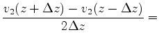
 are the horizontal wavenumbers and
  is a depth step,
  are Fourier-transforms of the three displacement components
  and
and  are their z-derivatives. At the boundaries
and
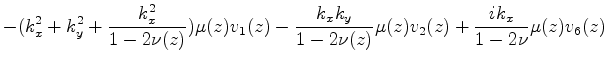
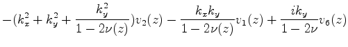
the central differences should be replaced with backward and forward differences (Iserles, 2008), and the boundary conditions 15 Fourier-transformed in a similar manner. In combination with the Fourier-transformed boundary conditions the above system is reduced to independent
are their z-derivatives. At the boundaries
and
the central differences should be replaced with backward and forward differences (Iserles, 2008), and the boundary conditions 15 Fourier-transformed in a similar manner. In combination with the Fourier-transformed boundary conditions the above system is reduced to independent
 linear systems for finding
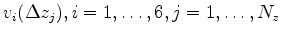 for each wavenumber pair
, where
for each wavenumber pair
, where  is the number of depth steps.
|
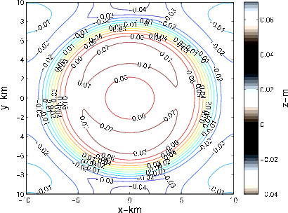
csubszdispoutsymhires
Figure 11. Contour plot of the displacements modelled from the axisymmetric pore pressure decline of Fig 2(a). |
|
|---|---|
|
|
|
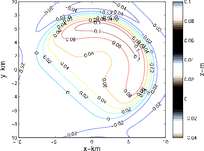
csubszdispoutasymhires
Figure 12. Contour plot of the displacements modelled from the asymmetric pore pressure decline of Fig 3(a). |
|
|---|---|
|
|
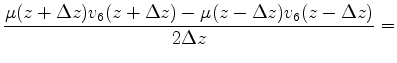
Solution of the above system is efficiently parallelized, with individual
sparse systems solved independently. Furthermore, each of the systems is banded with the bandwidth of 13 elements and therefore can be solved in a linear time and memory  (Trefethen and Bau, 1997).
Fig 11 and Fig 12 show the results of modeling surface subsidence from the axisymmetric and asymmetric pore pressure decline synthetics of Fig 2(a) and Fig 3(a). Here  with a 100 m depth step, the displacement field at the depth of 2 km was computed using operator 5. Although the above approach allows both elastic medium parameters (e.g., shear modulus
  and Poisson's ratio
  ) to be vertically heterogeneous, the latter, as the ratio of the axial and transverse strains, is usually less affected by compaction, and hence we left it constant at
  . However, the depth-dependent shear modulus is given by the formula
Although depth-varying models are common in geomechanical applications, and the diffusive nature of production-induced deformation favors slowly-varying models, there exist practical applications where strong lateral heterogeneity should be taken into account (for example, in subsalt regions). The widely accepted approach to tackling such problems consists of application of the finite elements method (Iserles, 2008) to the coupled poroelastic system (Kosloff et al., 1980). While finite elements can handle arbitrary spatial heterogeneity, the main disadvantage of this approach is the necessity to solve a potentially very large system of linear equations with very sparse but generally unstructured matrix.
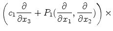
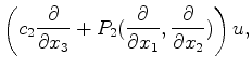
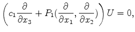
A possible extension of our approach for tackling arbitrary heterogeneity could be summarized as follows. If system 14 can be factorized
 and
and  are some pseudo-differential operators and
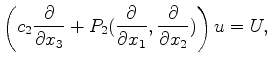
  are some functions, then given the boundary conditions 15, the boundary-value problem 14,15 can be solved by solving
 |
(19) |
, followed by solving
|
|
|
|
Identifying reservoir depletion patterns from production-induced deformations with applications to seismic imaging |


![$\displaystyle \frac{1}{1+\frac{1}{1-2\nu(z)}}\left[ -(k_x^2+k_y^2)v_3(z)+\frac{i k_x}{1-2 \nu(z)}v_4(z)+ \frac{i k_y}{1-2 \nu(z)}v_5(z)\right],$](img89.png)
![$\displaystyle {\nabla} \cdot \mu(x_1,x_2,x_3)\left[\left(\frac{\partial u_i}{\p...
...ght)+\frac{2 \nu}{1-2\nu}\frac{\partial u_k}{\partial x_k}\delta_{ij} \right] =$](img101.png)