Identifying reservoir depletion patterns from production-induced deformations with applications to seismic imaging

Modeling Displacements from Pore-Pressure Decline

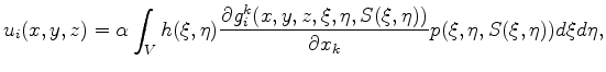
We can use operator 4 for forward-modeling the displacement field from a specified pressure change. Note that operator 4 is a non-stationary convolutional integral operator for a homogeneous medium. The convolution is non-stationary due to the presence of $z+\zeta$ in the elastostatic Green's tensor. Integration along the horizontal axes can be accelerated by applying the operator in the wavenumber domain. However, integration along the vertical axis should still be carried out separately for different values of $z$ , hence the integration kernel is effectively four-dimensional. Assuming the reservoir to be thin in comparison with its lateral extents, which is always the case, we can replace the vertical integral with a mean value of the integrand times the reservoir thickness:

$$u_i(x,y,z)=\alpha \int_V h(\xi,\eta)\frac{\partial g^k_i(x,y,z,\xi,\eta,S(\xi,\eta))}{\partial x_k}p(\xi,\eta,S(\xi,\eta)) d\xi d\eta,$$ (5)

where $S(\xi,\eta)$ is the middle surface of the reservoir and $h(\xi,\eta)$ is the reservoir depth. For a non-flat reservoir, $g^k_i$ effectively depends not only on differences $x-\xi$ and $y-\eta$ but on integration variables as well. In our implementation we compute 5 as a full convolutional operator, allowing slowly-varying asymptotics of the solutions by introducing scaling factors that depend on both $(x,y,z)$ and $(\xi,\eta,\zeta)$ .

An implementation of this method is provided by the poroelastic_green.F90 module of the author's exp_tk Fortran 2003 object-oriented framework described in Appendix B.

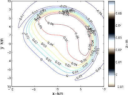
We test our approach on synthetic data generated for a reservoir model based on the assumed geometry of the gas reservoir near Lacq, France, described by Segall et al. (1994). The reservoir is assumed to be anticlinal dome-shaped, with the depth of the reservoir approximated as

$$D(\rho)=3.5-1.4\left( \exp{\left[\left(\frac{\rho}{5}\right)^2\right]}-.5\right),$$ (6)

where $\rho$ is the distance to the center of the reservoir, and all the distances are measured in km (see Fig 1). The reservoir thickness is estimated to be $\approx .35$ km. In the first test we apply the forward-modeling operator 5 to an axisymmetric synthetic pore pressure drop similar to the pore pressure change used by Segall et al. (1994) and given by

$$p(\rho)=55 \times \exp{\left[\left(\frac{\rho}{8}\right)^4\right]},$$ (7)

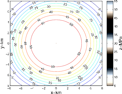
(see Fig 2(a)). The pressure in equation 7 and the rest of the paper is measured in MPa, and $\rho$ is the distance to the center of the reservoir. The result of displacement modeling using an $81\times 81$ reservoir grid and $101\times 101$ surface grid is shown on Fig 2(b). Linear poroelasticity predicts a linear relationship between the maximum subsidence and the maximum pore pressure decline. Segall et al. (1994) predicts that the subsidence rate for the axisymmetric model is bracketed between $.7$ mm/MPa for the reservoir thickness of $.25$ km and $1.37$ mm/MPa for the thickness of $.45$ km. The subsidence rate indicated by Fig 2(b) for the value of the reservoir thickness of $.35$ km is in a good agreement with that prediction. i

cppsymhires,csubsdispoutsymhires
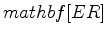
Figure 2. a) Contour plot of the axisymmetric pore pressure drop given by equation 7. b) Contour plot of the subsidence above the reservoir of Fig 1 due to the axisymmetric pore pressure decline of Fig 2(a).

Next, we apply the modeling operator to the asymmetric synthetic pore pressure drop given by

$$p(\rho)=55 \times \exp{\left[\left(\frac{\rho}{8(1+\sin{\phi-\pi/4})}\right)^4\right]},$$ (8)

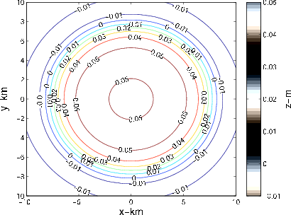
where $\rho,\phi$ are the distance and azimuth from an off-centre point (3 km,3 km), with a steeper decline in pore pressure along the northeast-southwest directions (see Fig 3(a)). The pressure decline given by equation 8 is not based on any specific real-world example but is rather chosen as a somewhat extreme case of an asymmetric pressure decline pattern mismatching the reservoir geometry. The result of modeling displacements due to the asymmetric pore pressure decline within the reservoir, using the same reservoir and surface grids as above, is shown on Fig 3(b).

cppasymhires,csubsdispoutasymhires
Figure 3. a) Contour plot of the asymmetric pore pressure drop given by equation 8. b) Contour plot of the subsidence above the reservoir of Fig 1 due to the asymmetric pore pressure decline of Fig 3(a).

The following table summarizes the medium parameters taken from (Segall et al., 1994) that are used in our tests:

Parameter	SI	Imperial
$\nu$	.25	dimensionless
$\alpha$	.25	dimensionless
$\mu$	$23.$ GPa	$3.34$ Mpsi

The Biot coefficient $\alpha$ is computed as

$$\alpha=1-\frac{K_{\texttt{und}}}{K_{\texttt{min}}},$$ (9)

with $K_{\texttt{und}},K_{\texttt{min}}$ being the undrained bulk modulus and the bulk modulus of rock mineral grains, respectively (Mavko et al., 2009).

Modeling subsidence using operator 5, we are able to fully account for the asymmetric nature of the depletion pattern by using the most general form of Green's tensor for a homogeneous half-space. In that respect, our approach represents an advancement of the purely analytical techniques for axisymmetric reservoirs presented in (Geertsma, 1973) and (Segall et al., 1994). However, the assumption of homogeneity, which is required for our being able to use analytical expressions for the Green's tensor, is a serious limitation that may significantly impair the applicability of our method, especially bearing in mind that our ultimate objective is to estimate subsurface displacements from observable subsidence. Later in the paper we propose a computationally efficient extension of our method that is capable of tackling heterogeneity.

Identifying reservoir depletion patterns from production-induced deformations with applications to seismic imaging