A new method for more efficient seismic image segmentation

Results

The results of the procedure detailed in the sections above can be seen in Figures 7(a) and 7(b). In Figure 7(a), although the salt body has been segmented into several regions, all of these regions are contained within the salt body and fully conform to its boundaries. This represents an improvement over the original segmentation in Figure 3(a). The improvement is even more dramatic for the field data example (original image in Figure 1(b)). In Figure 7(b), we see that the salt body has been segmented virtually perfectly; no longer do the salt body segments spill over the boundary, nor are parts of the boundary itself treated as individual segments as we saw in the original example.

zig-segfinal2,uno-segfinal2
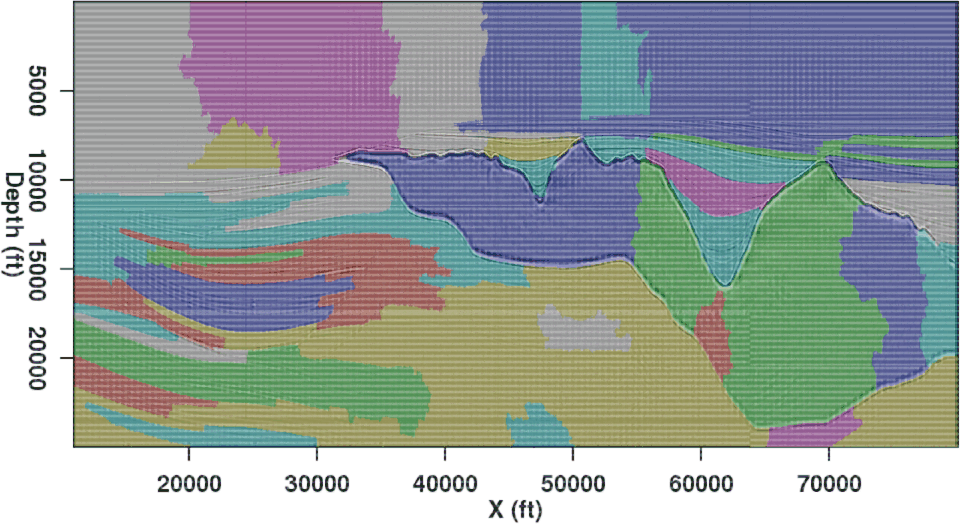
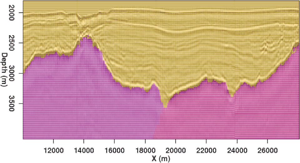
Figure 7. Results of applying the modified segmentation algorithm to the example images from Figure 1. Both (a) and (b) are a significant improvement over the original results in Figures 3(a) and 3(b).

A major motivation behind this research was to improve on segmentation results using the NCIS method from Shi and Malik (2000), and adapted for use with seismic images by Lomask et al. (2007). The first indication that the newer method does indeed represent a substantial improvement is the fact that the synthetic image from Figure 1(a) is simply too large to be segmented on a single processor using the existing NCIS implementation. The necessity of holding a giant, sparse weight matrix in memory and calculating an eigenvector precludes problems of this size from being feasible. The smaller field data example, however, is well-suited for the NCIS algorithm, and will allow us to make a relatively fair comparison. Figure 8(a) shows the eigenvector produced by the NCIS method to segment the image. In this case, the graph partition will occur between the negative (red) and positive (blue) values of the eigenvector. The boundary resulting from this partition is drawn on the image in Figure 8(b). Recall that in order to make the problem more computationally feasible, the computational domain is already limited around a ``prior guess'' of the boundary. The pairwise region comparison method developed here requires no such limitation, which is another indication of its superiority.

A new method for more efficient seismic image segmentation