|
|
|
|
A new method for more efficient seismic image segmentation |
| CPU time (s) | |||
| Image type | Pixels | NCIS | PRC |
| Synthetic data | 2761000 | n/a | 31 |
| Field data | 55000 | 156 | 1 |
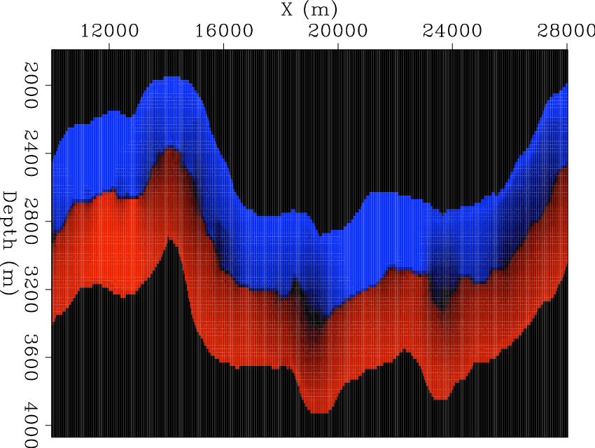
Again, due to memory constraints the existing NCIS implementation is unable to segment an image the size of Figure 1(a). The implementation described here, however, produces an accurate segmentation in 31 seconds; during this time, approximately 55 million edges are created, weighted, and used to segment the graph. The efficiency advantage for the new implementation is quantified using the field data example; in this case, the image is segmented over 150 times faster using the new implementation. These differences are extremely significant and represent a huge savings of time and computational expense, especially for larger problems.
|
|---|
|
uno-eig,uno-segeig
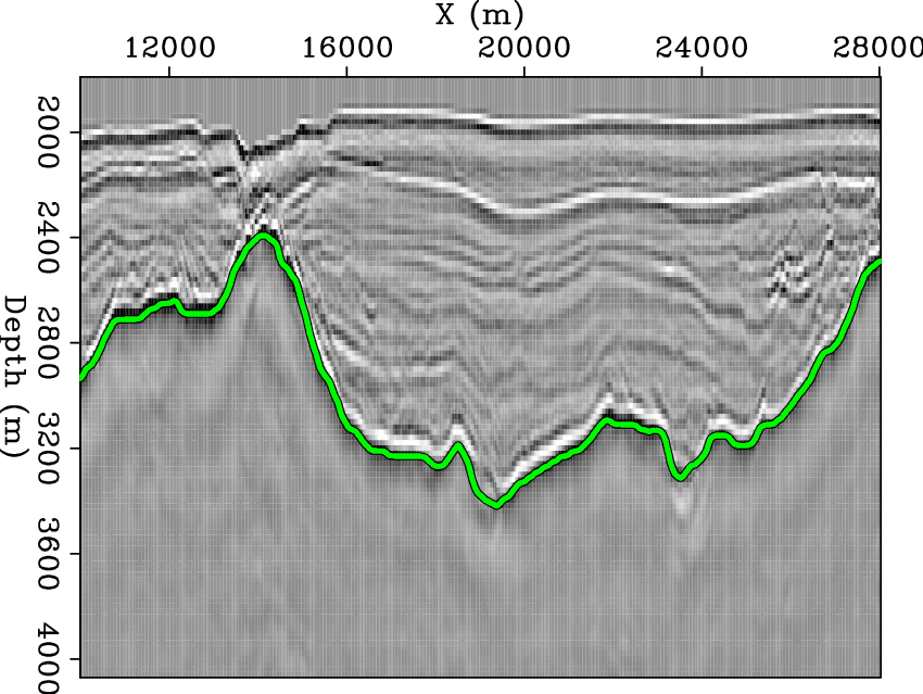
Figure 8. Eigenvector (a) used to segment the image in Figure 1(b) according to the NCIS algorithm of Shi and Malik (2000) and adapted for seismic data by Lomask et al. (2007), and the resulting salt boundary (b). |
|
|
|
|
|
|
A new method for more efficient seismic image segmentation |