next up previous [pdf]

Next: Creating the graph Up: Approach Previous: Data input and manipulation

Transformation of input data

Seismic data may be thought of as signals with amplitude and phase varying as a function of time (or depth). This could present problems for any segmentation algorithm, and we may see an indication of this in Figure 3(b). At the boundary between the salt body and the surrounding rocks, the seismic waves change phase rapidly; this is common behavior when the waves encounter an interface and reflect back to the surface. As originally written, the algorithm may interpret the area around the boundary as several regions, instead of an interface between just two regions. In this case, the boundary itself becomes its own ``region'' in several locations. To avoid this situation, we would like the seismic image to be represented as amplitude information only, since this would indicate a single boundary between two regions. As Taner et al. (1979) point out, seismic data may be represented as a complex valued function:

$\displaystyle A(z)e^{i\phi(z)},$ (4)

where $ z$ can be time or depth. The exponential term in this expression represents the phase information for the seismic data, while the leading term represents the amplitude information. By transforming the data such that the amplitude information is the only information present, the problem described above may be avoided. Figures 4(a) and 4(b) show the result of this process, also known as taking the ``amplitude of the envelope'' of the data, for the synthetic and field seismic images, respectively. We see that in both instances the phase information is no longer present, and the boundaries delineating the salt bodies are more clearly visible. By using these transformed images as inputs to the segmentation algorithm, it is likely that much of the unwanted behavior seen in the original examples can be avoided.

zig-origseg uno-origseg3
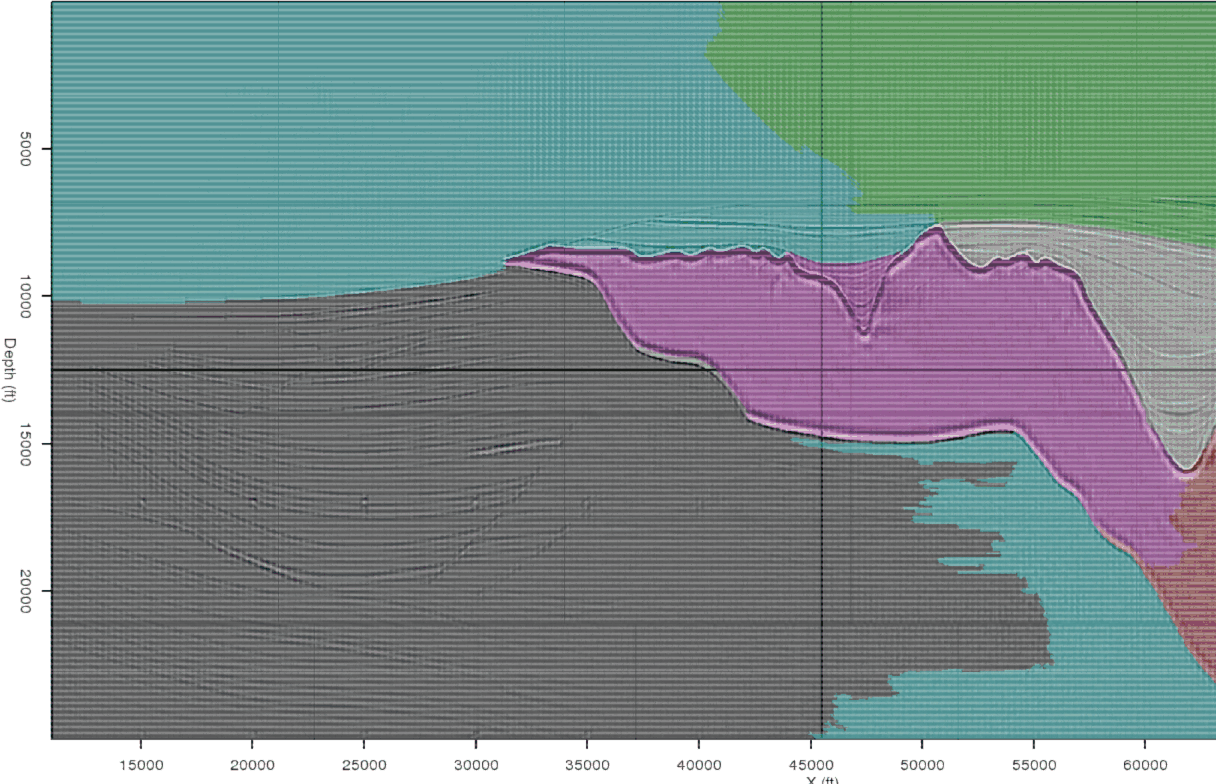
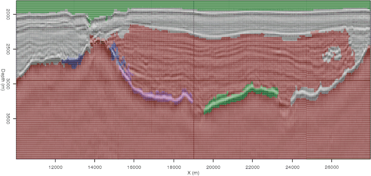
zig-origseg,uno-origseg3
Figure 3.
Segmentation of the example seismic images from Figure 1, using the original algorithm from Felzenszwalb and Huttenlocher (2004).
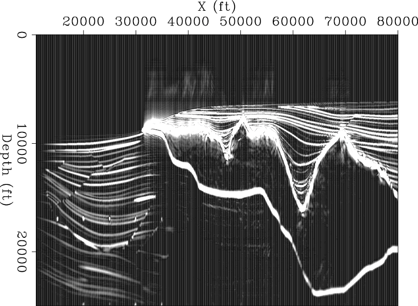
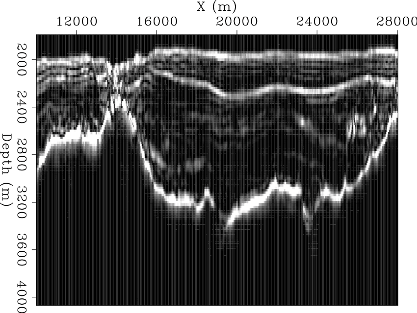
[pdf] [pdf] [png] [png]

zig-env uno-env
zig-env,uno-env
Figure 4.
Result of calculating the amplitude envelope of the example images seen in Figure 1. These become the input to the new segmentation algorithm.
[pdf] [pdf] [png] [png]


next up previous [pdf]

Next: Creating the graph Up: Approach Previous: Data input and manipulation

2010-05-19