A new method for more efficient seismic image segmentation

Calculating edge weights

The previous section details the construction of a graph used for segmentation of seismic images containing 40 edges per pixel. However, perhaps the most important part of any graph-based segmentation scheme is the calculation of weights for each of these edges. It is in this aspect that the algorithm described here differs most from the original implementation provided by Felzenszwalb (2010).

When using the original stencil seen on the left in Figure 5, determining edge weights is relatively straightforward. Since each pair of vertices are at most one pixel apart in the image, we can simply compare the adjacent pixel values and use some expression to determine the likelihood that the two pixels reside in different regions or segments. This process is further simplified by the fact that the original implementation was designed to segment regions with coherent interiors; that is, even if the interior of a region is relatively chaotic, it is still distinct from the interiors of other regions of the image. However, this is not necessarily the case for seismic images - the interior of a salt body might not be distinct from other areas in the image that lack reflections. In this case a region is defined by its boundary rather than the character of its interior. Therefore, we must create a process for calculating edge weights that treats a boundary between two vertices as more convincing evidence for the existence of two regions than simply the difference in intensity at the two pixels themselves.

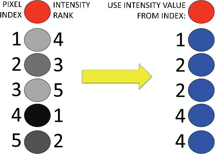
As described in the previous section, the stencil used for determining graph edges forms what are essentially four line ``segments'' at each vertex - one horizontal, one vertical, and two diagonal. Recall that once the entire graph is constructed, each vertex will actually be connected with eight such segments due to reciprocity of the calculations. Since two vertices that are the endpoints of a graph edge are no longer necessarily adjacent in the image, determining the existence of a boundary between them is no longer straightforward. However, the construction of distinct line segments extending from each pixel suggests one method of searching for a boundary: existence of a large amplitude value at any point along the line segment between the two pixels comprising the edge is evidence of a boundary. In other words, the intensity values of the two vertex pixels themselves will not be used to determine the edge weight; rather, the largest intensity value of any pixel along the line segment connecting the two endpoint vertices will be used. This strategy follows the approach of Lomask (2007) in his NCIS implementation. Figure 6 illustrates the logic behind this process. If all pixels in a segment are ranked according to intensity, the highest ranked pixel between the two edge vertices will be used for the weight calculation.

pixels Figure 6. Diagram illustrating the logic behind deciding which pixel intensity value to use when calculating edge weights. Pixel intensities are shown and ranked on the left; the numbers in the right column indicate which intensity value will be used when calculating the edge weight between the pixel in red and the adjacent blue pixel.

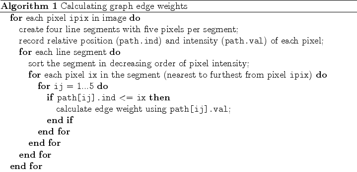
This process obviously involves some degree of algorithmic complexity, as it requires sorting and searching the pixel intensity values along each segment. Algorithm 5 illustrates the steps for carrying out the process shown graphically in Figure 6. After creating the edges linking each pixel in a line segment to the ``active'' pixel, sort the line segment's pixels in decreasing order of pixel intensity. Once this is done, compare the index value of the edge vertex pixel with the intensity-ranked list of pixel indices. To find the highest-intensity pixel value between the two vertices, simply take the value of the first pixel index on the sorted list that is less than the index of the vertex pixel.

Once we have selected the intensity value to use for determining the edge weight, we must still calculate the weight value itself. The original implementation from Felzenszwalb (2010) used a simple Euclidean ``distance'' between adjacent pixel values. For RGB images, this expression is the equivalent of taking the square root of the sum of the squared differences for each of the three color components at each pixel. However, for the purposes of seismic image segmentation I have found it more appropriate to use an exponential function:

$$w_{ij} = \exp ((\max I({\bf p}_{ij}))^2),$$ (5)

where ${\bf p}_{ij}$ is the vector of all pixels between $i$ and $j$ . Additionally, since the edges in the graph can now be much longer than with the adjacent-pixels-only approach taken in the original implementation, it makes sense to include a distance-weighting term to the edge weight calculation:

$$w_{ij} = \exp ((\max I({\bf p}_{ij}))^2) \exp (d_{ij}),$$ (6)

where $d_{ij}$ is simply the Euclidean distance (in samples) between the two pixels.

Once each of the edges is assigned a weight, the segmentation of the image can proceed as described in Felzenszwalb and Huttenlocher (2004). In summary, the process begins with each pixel as its own image segment; then individual pixels, and eventually, groups of pixels, are merged according to the criteria set forth in section 2. Segments can also be merged in post-processing if they are smaller than a ``minimum segment size'' parameter specified by the user.

A new method for more efficient seismic image segmentation