Delayed-shot migration in TEC coordinates

Inline delayed-shot migration

An alternate 3D migration formulation is to phase-encode individual sail lines for a given ray parameter, 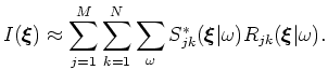$p_{\xi_1}$, solely according to inline source position. This phase-encoding approach is related to conical-wave migration, which requires $j-l=0$ in equation 3. However, I choose to not make this restriction because it is realized only by straight sail lines and non-flip-flop sources (Liu et al., 2006). Rather, I present an alternative theory of inline delayed-shot migration that allows more general crossline source and receiver distribution.

Inline delayed-shot wavefields, propagated through the migration domain to generate the full source and receiver wavefield volumes, are defined by

$$\overline{S(\boldsymbol{\xi}\vert\omega )}= \sum_{l=1}^A \sum_{j=... ...\xi}\vert\omega ) f(\omega ) {\rm e}^{ i\omega [p_{\xi_1} \Delta \xi_1 (j-p)]},$$ (7)

$$\overline{R(\boldsymbol{\xi}\vert\omega )}= \sum_{l=1}^A \sum_{k=... ...xi}\vert\omega ) f(\omega ) {\rm e}^{ i \omega [p_{\xi_1} \Delta \xi_1 (k-p)]},$$ (8)

where $j$ and $k$ are the source and receiver inline position, respectively, $B$ is the number of inline records, $l$ is the sail line index out of a total of $A$ sail lines, and $p$ is a reference inline index.

An image volume $I(\boldsymbol{\xi})$ is generated from a series of inline delayed-shot migration images, $I_l^{DS}(\boldsymbol{\xi}\vert p_{\xi_1})$, formed by correlating the composite inline source and receiver wavefields and stacking the results over frequency. The inline delayed-shot migration kernel mixes source and receiver wavefield energy, $S_{jl}(\boldsymbol{\xi}\vert\omega )$ and $R_{kl}(\boldsymbol{\xi}\vert\omega )$, according to

$$I(\boldsymbol{\xi}) = \sum_{l=1}^A \sum_{p_{\xi_1}} \sum_{j=1}^B \sum_{k=1}^B I^{DS}_{jkl}(\boldsymbol{\xi}\vert p_{\xi_1})$$ (9)

$$ = \sum_{l=1}^A \sum_{p_{\xi_1}} \sum_{j=1}^B \sum_{k=1}^B \sum_{\om... ...ldsymbol{\xi}\vert\omega ) {\rm e}^{ i \omega [ p_{\xi_1} \Delta \xi_1 (j-k)]},$$

Similar to plane-wave migration, mixing wavefields of differing 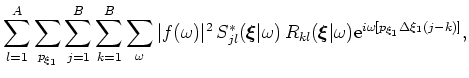$S_{jl}$ and $R_{kl}$ indices will introduce crosstalk into the image volume. However, inline delayed-shot migration will be crosstalk-free in the following limit:

$$\lim_{N_{p_{\xi_1}} \rightarrow \infty} \sum_{\alpha = -N_{p_{\xi... ... \Delta p_{\xi_1} \Delta {\xi_1} (j-k) } = \vert \omega \vert^{-1} \delta_{jk},$$ (10)

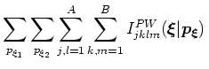
Defining $\vert f(\omega )\vert^2=\vert\omega \vert$ and using the approximation in equation 10, I rewrite

$$I_l^{DS}(\boldsymbol{\xi}) \approx \sum_{j=1}^B \sum_{\omega }S_{jl}^*(\boldsymbol{\xi}\vert\omega ) R_{jl}(\boldsymbol{\xi}\vert\omega ).$$ (11)

Stacking over all inline delayed-shot sail-line migration results yields the full image volume,

$$I(\boldsymbol{\xi}) \approx \sum_{l=1}^A I_l^{DS}(\boldsymbol{\xi... ...a }S_{jl}^*(\boldsymbol{\xi}\vert\omega ) R_{jl}(\boldsymbol{\xi}\vert\omega ).$$ (12)

This proves the equivalence of inline delayed-shot and shot-profile migration.

Delayed-shot migration in TEC coordinates