Delayed-shot migration in TEC coordinates

Full plane-wave phase-encoding migration

Performing 3D plane-wave migration is similar in many respects to 3D shot-profile migration. The main differences derive from how the composite source and receiver wavefield volumes, $\overline{S}$ and $\overline{R}$, are re-synthesized from individual source and receiver profiles, $S_{jk}$ and $R_{lm}$, prior to imaging. The complete wavefields are generated by filtering the source and receiver profiles by a function dependent on the inline and cross-line plane-wave ray parameters, $\boldsymbol{p_\xi}=[p_{\xi_1}, p_{\xi_2}]$. These wavefields are then propagated through the migration domain to generate the full source and receiver wavefield volumes

$$\overline{S(\boldsymbol{\xi}\vert\omega )}= \sum_{j=1}^A \sum_{k=... ...m e}^{ i\omega [p_{\xi_1} \Delta \xi_1 (j-p) + p_{\xi_2} \Delta \xi_2 (k-q) ]},$$ (1)

$$\overline{R(\boldsymbol{\xi}\vert\omega )}= \sum_{l=1}^A \sum_{m=... ...m e}^{ i\omega [p_{\xi_1} \Delta \xi_1 (l-p) + p_{\xi_2} \Delta \xi_2 (m-q) ]},$$ (2)

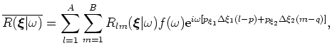where $f(\omega )$ is a frequency filter to be discussed below, $\Delta \xi_1$ and $\Delta \xi_2$ are the inline and cross-line sampling intervals, $p$ and $q$ are reference spatial indices in the inline and cross-line directions, $j$ and $k$ are indices fixing the inline and crossline source position, $l$ and $m$ are indices fixing the inline and cross-line receiver position, and $A$ and $B$ are the number of inline and cross-line source records, respectively. The phase encoding, implemented at the surface independent of wavefield extrapolation, is valid for any generalized coordinate system. Note that the wavefield propagation throughout the migration volume in equations 1 and 2 is understood, and assumed to be governed by the wavefield propagation techniques described in Shragge (2008).

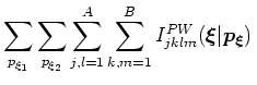
An image volume $I(\boldsymbol{\xi})$ is formed from a series of individual full plane-wave migration images, $I^{PW}(\boldsymbol{\xi}\vert \boldsymbol{p_{\xi}})$, by correlating the composite plane-wave source and receiver wavefields and stacking the results over frequency. The plane-wave migration kernel mixes source and receiver wavefield energy, $S_{jk}(\boldsymbol{\xi}\vert\omega )$ and $R_{lm}(\boldsymbol{\xi}\vert\omega )$, according to

$$I(\boldsymbol{\xi}) = \sum_{p_{\xi_1}} \sum_{p_{\xi_2}} \sum_{j,l=1}^A \sum_{k,m=1}^B I^{PW}_{jklm}(\boldsymbol{\xi}\vert \boldsymbol{p_\xi})$$ (3)

$$ = \sum_{p_{\xi_1}} \sum_{p_{\xi_2}} \sum_{j,l=1}^A \sum_{k,m=1}^B \... ...e}^{ i \omega [ p_{\xi_1} \Delta \xi_1 (j-l) + p_{\xi_2} \Delta \xi_2 (k-m) ]},$$

where 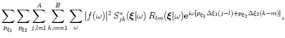$^*$ indicates complex conjugate.

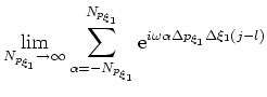
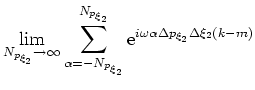
Generally, mixing wavefields of differing $S_{jk}$ and $R_{lm}$ indices introduces image crosstalk. A plane-wave migration image will be crosstalk-free, though, in the following limits:

$$\lim_{N_{p_{\xi_1}} \rightarrow \infty} \sum_{\alpha = -N_{p_{\xi... ...N_{p_{\xi_1}}}{\rm e}^{ i \omega \alpha \Delta p_{\xi_1} \Delta {\xi_1} (j-l) } = \vert\omega \vert^{-1} \delta_{jl},$$

$$\lim_{N_{p_{\xi_2}} \rightarrow \infty} \sum_{\alpha = -N_{p_{\xi... ...N_{p_{\xi_2}}}{\rm e}^{ i \omega \alpha \Delta p_{\xi_2} \Delta {\xi_2} (k-m) } = \vert\omega \vert^{-1} \delta_{km}.$$ (4)

where $N_{p_{\xi_1}}$ and $N_{p_{\xi_2}}$ are the number of plane waves in the $\xi _1$ and $\xi _2$ directions. Assuming that equation 4 approximately is valid (i.e., for large values of $N_{p_{\xi_1}}$ and $N_{p_{\xi_2}}$), I rewrite equation 3 as

$$I(\boldsymbol{\xi}) \approx \sum_{j=1}^A \sum_{k=1}^B \sum_{\omeg... ...2} S_{jk}^*(\boldsymbol{\xi}\vert\omega ) R_{jk}(\boldsymbol{\xi}\vert\omega ),$$ (5)

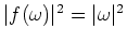
which, by defining 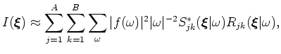$\vert f(\omega )\vert^2=\vert\omega \vert^2$, generates the following expression:

$$I(\boldsymbol{\xi}) \approx \sum_{j=1}^M \sum_{k=1}^N \sum_{\omega } S_{jk}^*(\boldsymbol{\xi}\vert\omega ) R_{jk}(\boldsymbol{\xi}\vert\omega ).$$ (6)

This demonstrates the equivalence between plane-wave and shot-profile migration (Liu et al., 2006).

Delayed-shot migration in TEC coordinates