|
|
|
|
Angle-domain common-image gathers in generalized coordinates |
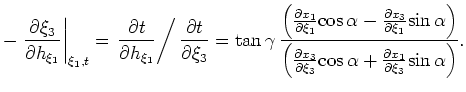
Answering this question requires properly formulating the derivative operators,
![]() and
and
![]() , in equations 7 in the generalized coordinate system variables
, in equations 7 in the generalized coordinate system variables
![]() and
and
![]() . Appendix A shows how these derivatives can be specified using Jacobian change-of-variable arguments. Assuming that the subsurface-offset axes are formed by uniform wavefield shifts, such that the geometries of
. Appendix A shows how these derivatives can be specified using Jacobian change-of-variable arguments. Assuming that the subsurface-offset axes are formed by uniform wavefield shifts, such that the geometries of
![]() and
and
![]() are equivalent Appendix A derives the following expression for generalized coordinate ADCIGs:
are equivalent Appendix A derives the following expression for generalized coordinate ADCIGs:
Similar to Cartesian coordinates, elliptic coordinate ADCIGs become insensitive where structural dips cause
 . However, this insensitivity can be minimized when using generalized coordinate systems, because structural dips appear at different angles in different translated elliptic meshes. Figures 2c-d illustrate this by showing a different coordinate shift for a different shot-location than that presented in panels 2a-b. Note the changes in structural dip in the right-hand-side of the elliptic coordinate panels. Thus, while ADCIGs calculated on one elliptic grid may be insensitive to certain structure locally, mesh translation ensures that ADCIGs are sensitive globally. Imaging steep dips in elliptic coordinates, though, is limited by the accuracy of wide-angle one-way wavefield extrapolation.
Finally, one may calculate reflection opening angles in the wavenumber domain for coordinate systems satisfying equations 11
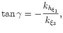 and and
|
|
|
|
Angle-domain common-image gathers in generalized coordinates |