Angle-domain common-image gathers in generalized coordinates

Generating subsurface offsets axes

Shot-profile migration in Cartesian coordinates consists of completing a recursive two-step procedure. The first step involves propagating the source and receiver wavefields, $S$ and $R$, from depth level $x_3-\Delta x_3$ to $x_3$ using an extrapolation operator $E_{x_3}[\cdot]$

$$E_{x_3}[S(x_3-\Delta x_3,x_1\vert\omega)] = S(x_3,x_1\vert\omega),$$

$$E^*_{x_3}[R(x_3-\Delta x_3,x_1\vert\omega)] = R(x_3,x_1\vert\omega),$$ (1)

where 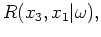$*$ denotes the conjugate operator, $\omega$ is angular frequency, and $\Delta x_3$ is the depth step. A subsurface image, $I$, is subsequently computed at each extrapolation step by evaluating an imaging condition

$$I(x_3,x_1,h_{x_1}) = \sum_\omega S^*(x_3,x_1-h_{x_1}\vert\omega) R(x_3,x_1+h_{x_1}\vert\omega),$$ (2)

where the subsurface-offset axis, $h_{x_1}$, is generated by correlating the source and receiver wavefields at various relative shifts in the 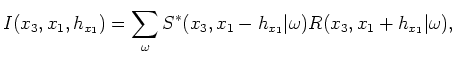$x_1$ direction. Finally, the ADCIG volume is computed using an offset-to-angle transformation operator, ${\bf T}_{h_{x_1} \rightarrow \gamma}$

$$I(x_3,x_1,\gamma) = {\bf T}_{h_{x_1}\rightarrow \gamma} I(x_3,x_1,h_{x_1}),$$ (3)

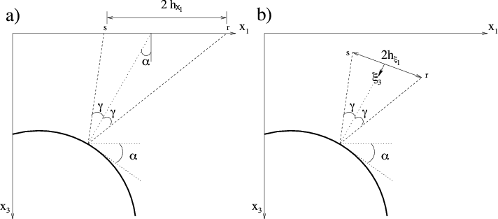
where $\gamma$ is the reflection opening angle shown in Figure 1.

rays
Figure 1. Cartoon illustrating the geometry of the ADCIG calculation. Parameter $\gamma$ is the reflection opening angle, $\alpha$ is geologic dip. a) Cartesian geometry using coordinates $x_1, x_3$ and$h_{x_1}$. b) Generalized geometry using coordinates $\xi _1, \xi _3$ and $h_{\xi _1}$. Adapted from ().

Imaging in generalized coordinate systems follows the same two-step procedure. However, because of the different migration geometry in the $\boldsymbol{\xi}$-coordinate system, new extrapolation operators, $E_{\xi_3}[\cdot]$, must be used to propagate wavefields. I specify these operators using Riemannian wavefield extrapolation (RWE). I do not discuss RWE herein, and refer readers interested in additional information to () and ().

The first generalized coordinate imaging step is performing wavefield extrapolation

$$E_{\xi_3}[S(\xi_3-\Delta \xi_3,\xi_1\vert\omega)] = S(\xi_3,\xi_1\vert\omega),$$

$$E^*_{\xi_3}[R(\xi_3-\Delta \xi_3,\xi_1\vert\omega)] = R(\xi_3,\xi_1\vert\omega),$$ (4)

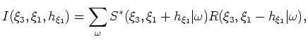
where $\Delta \xi_3$ is the extrapolation step increment. Generalized coordinate images are then constructed by evaluating an imaging condition

$$I(\xi_3,\xi_1,h_{\xi_1}) = \sum_\omega S^*(\xi_3,\xi_1 + h_{\xi_1}\vert\omega) R(\xi_3,\xi_1 - h_{\xi_1}\vert\omega),$$ (5)

where $h_{\xi _1}$ is the $\boldsymbol{\xi}$-coordinate equivalent of Cartesian subsurface offset axis $h_{\xi _1}$. The generalized coordinate ADCIG volume is generated by applying an offset-to-angle transformation ${\bf T}_{h_{\xi}\rightarrow\gamma}$

$$I(\xi_3,\xi_1,\gamma) = {\bf T}_{h_{\xi_1}\rightarrow \gamma} I(\xi_3,\xi_1,h_{\xi_1}).$$ (6)

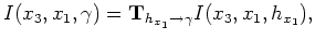
Conventional ADCIG volumes can be recovered by sinc interpolating each 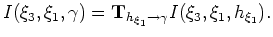$I(\xi_3,\xi_1,\gamma)$ image computed via equation 6 to the final Cartesian coordinate volume.

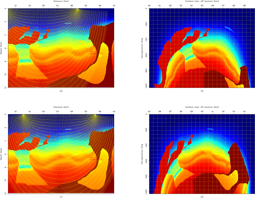
Figure 2 illustrates this process using the elliptic coordinate system. Panel 2a shows the BP synthetic velocity model (, ) with an elliptic mesh overlain. Note that the salt flanks to the right-side of the model are nearly vertical in Cartesian coordinates. Panel 2b shows the velocity model in panel 2a interpolated to the elliptic coordinate system. Importantly, the aforementioned salt flanks in the elliptic coordinate system are nearly horizontal, which should lead to ADCIG calculations more robust than in Cartesian coordinates. However, proving this assertion requires understanding the differences, if any, between the Cartesian and generalized coordinate offset-to-angle operators, ${\bf T}_{h_{x_1} \rightarrow \gamma}$ and ${\bf T}_{h_{\xi_1}\rightarrow \gamma}$, in equations 3 and 6, respectively.

RC2
Figure 2. Prestack migration test in elliptic coordinates. a) Benchmark synthetic velocity model with an overlying elliptic coordinate system. b) Effective slowness model in the transformed elliptic coordinate system in a). c) Benchmark synthetic velocity model with a different overlying elliptic coordinate system. d) Effective elliptic coordinate slowness model for the coordinate system in c).

Angle-domain common-image gathers in generalized coordinates