|
|
|
|
Joint wave-equation inversion of time-lapse seismic data |
In principle, it is possible to solve for a least-squares solution to equation 13 by minimizing the cost function
As discussed in the JID formulation, this would be too expensive to be practical since the cost of one iteration is at least the cost of four migrations. Ajo-Franklin et al. (2005) have shown a tomographic example of this formulation, but since each migration is orders of magnitudes more expensive than ray-based tomography, this approach would be too expensive for wave-equation inversion. Therefore, we reformulate equation 14 as
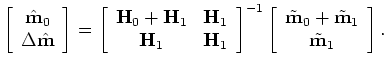 and
and
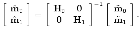 respectively) can be obtained from equation 17 and the time-lapse image as a difference between the two images as done in equation 5.
Also, note that without coupling, as done in the next section, equation 16 is equivalent to equation 5.
Since the Hessian matrices
respectively) can be obtained from equation 17 and the time-lapse image as a difference between the two images as done in equation 5.
Also, note that without coupling, as done in the next section, equation 16 is equivalent to equation 5.
Since the Hessian matrices
|
|
|
|
Joint wave-equation inversion of time-lapse seismic data |
![\begin{displaymath}\begin{array}{ccc} S({\bf m_0}, {\bf m_1})= \left \vert\left\...
...end{array} \right ] \right \vert \right \vert ^2. \end{array}\end{displaymath}](img51.png)
![$\displaystyle \left [ \begin{array}{cc} {\bf L'}_{0} {\bf L}_{0} & {\bf0} {\...
...begin{array}{cc} \tilde {\bf m}_{0} \tilde {\bf m}_{1} \end{array} \right ],$](img52.png)
![$\displaystyle \left [ \begin{array}{ccc} {\bf H}_{0} & {\bf0} {\bf0} & {\bf ...
...begin{array}{cc} \tilde {\bf m}_{0} \tilde {\bf m}_{1} \end{array} \right ],$](img53.png)
![$\displaystyle \left [ \begin{array}{cc} \hat{{\bf m}}_{0} \hat{{\bf m}}_{1} ...
...begin{array}{cc} \tilde {\bf m}_{0} \tilde {\bf m}_{1} \end{array} \right ].$](img54.png)