Joint wave-equation inversion of time-lapse seismic data

Joint-inversion for image differences (JID)

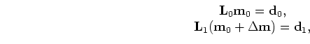
First, we re-formulate the data modeling operations for the two surveys in equation 2 as follows:

$$\begin{array}{cc} {\bf L}_{0} {\bf m}_{0} = {\bf d}_{0}, {\... ...}_{1}({\bf m}_{0} + \Delta {\bf m} ) = {\bf d}_{1}, \end{array}$$ (A-7)

where ${\bf m}_{0} + \Delta {\bf m} = {\bf m}_{1}$. In matrix form, these expressions can be combined to give

$$\left [ \begin{array}{cc} {\bf L}_{0} & {\bf0 } {\bf L}_{1} & ... ... ] = \left [ \begin{array}{cc} {\bf d}_{0} {\bf d}_{1} \end{array} \right ].$$ (A-8)

In principle, using an iterative solver, a least-squares solution to equation 8 can be obtained by minimizing the cost function

$$\begin{array}{ccc} S({\bf m_0}, \Delta {\bf m})= \left \vert\... ...end{array} \right ] \right \vert \right \vert ^2. \end{array}$$ (A-9)

The computational cost of this approach is proportional to the number of iterations times at least twice the cost of one set of migrations -- since each iteration requires at least one modeling and one migration for the baseline and monitor datasets. Since several iterations would typically be required to reach convergence, and the inversion process would usually be repeated several times to fine-tune inversion parameters, the overall cost of this scheme will be high. An important advantage of the JID (or JMI) formulation is that modifications can be made to inversion parameters and the inversion repeated several times without the need for new migration or modeling. The least-squares solution to equation 8 is given by

$$\left [ \begin{array}{cc} {\bf L'}_{0} {\bf L}_{0}+{\bf L'}_{1} {... ...de {\bf m}_{0} + \tilde {\bf m}_{1} \tilde {\bf m}_{1} \end{array} \right ],$$ (A-10)

or

$$\left [ \begin{array}{ccc} {\bf H}_{0}+{\bf H}_{1} & {\bf H}_{1} ... ...de {\bf m}_{0} + \tilde {\bf m}_{1} \tilde {\bf m}_{1} \end{array} \right ],$$ (A-11)

which can be recast as

$$\left [ \begin{array}{cc} \hat{{\bf m}}_{0} \Delta \hat{{\bf m... ...de {\bf m}_{0} + \tilde {\bf m}_{1} \tilde {\bf m}_{1} \end{array} \right ].$$ (A-12)

Thus, the inverted baseline and time-lapse images ( 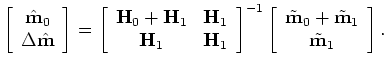${\hat{{\bf m}}}_{0}$ and $\Delta {\hat{{\bf m}}}$ respectively) can be obtained from equation 12. However, since the Hessian matrices ${\bf H}_{0}$ and ${\bf H}_{1}$ (and hence the joint Hessian operator) are not invertible, equation 11 is solved iteratively. We have extended equation 11 to multiple surveys (Appendix A). When multiple surveys are available, the outputs of the JID formulation are the inverted baseline image and image differences between successive surveys.

Joint wave-equation inversion of time-lapse seismic data