Waveform Inversion Problem

The goal of waveform inversion is to invert for the optimal set of velocity perturbations that minimize the difference between forward-modeled waveforms and acquired data. The first step in setting up the inverse problem is defining data residuals, $\Delta \Psi$,

$$\Delta \Psi({\mathbf r},{\mathbf s};\omega) = \Psi_m({\mathbf r},{\mathbf s};\omega) - \Psi_d({\mathbf r},{\mathbf s};\omega),$$ (18)

where $\Psi_d({\mathbf r},{\mathbf s})$ is the recorded data. The L₂ residual norm is used to set up an objective function,  

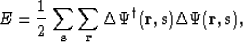$$E = \frac{1}{2} \sum_{{\mathbf s}} \sum_{{\mathbf r}} \Delta... ...({\mathbf r},{\mathbf s}) \Delta \Psi({\mathbf r},{\mathbf s}),$$ (19)

that is minimized with respect to slowness perturbations $\Delta s^ \dag$ 

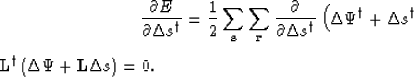$$\frac{\partial E}{\partial \Delta s^ \dag } = \frac{1}{2} \... ... \dag \right)\left(\Delta \Psi+ \mathbf{L}\Delta s\right)= 0.$$ (20)

This results in the following least-squares estimate of the slowness perturbations  

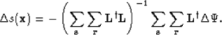$$\Delta s({\bf x}) = - \left(\sum_{{\mathbf s}} \sum_{{\mathb... ...{{\mathbf s}} \sum_{{\mathbf r}} \mathbf{L}^ \dag \Delta \Psi.$$ (21)

From here on, the sum over all sources and receivers is implicitly assumed. Also, we discuss only the gradient vector and the filtering of the gradient by the inverse Hessian matrix $\left(\mathbf{L}^ \dag \mathbf{L}\right)^{-1}$is implicitly assumed.

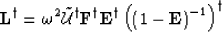
The adjoint gradient operator $\mathbf{L}^ \dag$ is a composite matrix consisting of a number of chained operators (from equation 16):

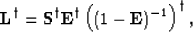$$\mathbf{L}^ \dag = \S^ \dag {\mathbf E}^ \dag \left((1 - {\mathbf E})^{-1} \right)^ \dag ,$$ (22)

where scattering operator or at each extrapolation interval, S_z is defined by (see Appendix A),

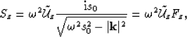$$S_z = \omega^2 \tilde{{\cal U}_z} \frac { {\rm i} s_0} {\sq... ... - \vert\mathbf{k}\vert^2 }} = \omega^2 \tilde{{\cal U}_z} F_z,$$ (23)

where $\mathbf F_z$ is considered a filter. This allows us to write composite operator $\mathbf{L}^ \dag$ with scattering ${\bf S}^ \dag$ and filter ${\bf \mathbf F}^ \dag$ matrices as,

$$\mathbf{L}^ \dag = \omega^2 \tilde{{\mathcal U}}^ \dag \ma... ...}^ \dag \left(\left(1 - {\mathbf E}\right) ^{-1}\right)^ \dag$$ (24)

Inserting this expression into equation 22 yields,

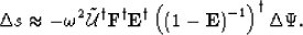$$\Delta s\approx -\omega^2 \tilde{{\mathcal U}}^ \dag \mathb... ...(\left(1 - {\mathbf E}\right) ^{-1}\right)^ \dag \Delta \Psi.$$ (25)

Thus, using the relationship in equations 6 and 7, leads to the following result,  

$$\Delta s\approx -\omega^2 {\mathbf G}_0^ \dag ({\bf x},{\ma... ...g ({\bf x},{\mathbf r}) \Delta \Psi({\mathbf r},{\mathbf s}).$$ (26)

 

• Relationship to Pratt's approach to waveform inversion