


Next: Limiting flattening model space
Up: R. Clapp: Moveout analysis
Previous: Flattening Review
There are two general approaches to calculating moveout parameters
using the flattening methodology. The first approach is to
perform parameter estimation in two phases. First, solve for the
non-linear  field, then construct a linear
problem to find the moveout parameters that best fit the
 field.
The flattening algorithm provides a time-shift  field
that is function of depth z, offset h, and CRP
  . As a first test
we want to estimate moveout of a volume migrated using downward continuation
migration. Biondi and Symes (2003) demonstrated that residual moveout
  can be approximated (assuming zero geologic dip)
as a function of angle
  and depth z through
|  |
(7) |
where  is the moveout paremeter.
We can estimate
  as a global inverse problem. Defining
the above moveout equation above as
  mwe obtain the objective function Q,
|  |
(8) |
We can ensure spatial smoothness by introducing a roughener  to the objective function to obtain,
|  |
(9) |
where  is scaling parameter.
To test the methodology I migrated a line from a 3-D North Sea dataset.
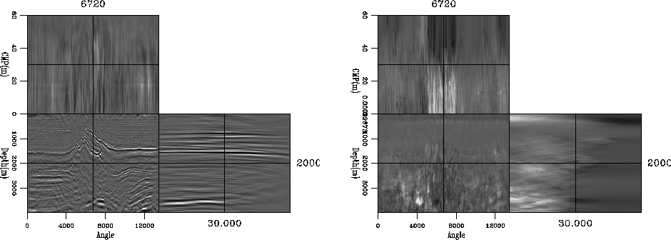
Figure ![[*]](http://sepwww.stanford.edu/latex2html/cross_ref_motif.gif) displays two cross-sections of the migrated
data (left) and the
displays two cross-sections of the migrated
data (left) and the  field (right) calculated from the volume.
A moveout field
  is then calculated from the
 field using a conjugate gradient algorithm to minimize
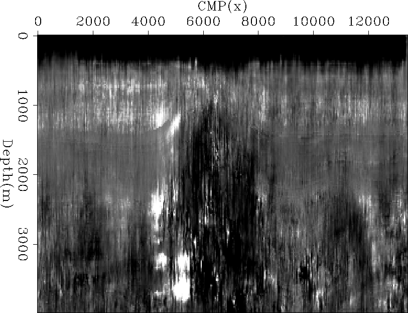
equation 9. Figure
 ![[*]](http://sepwww.stanford.edu/latex2html/cross_ref_motif.gif) shows the resulting
moveout field. The inversion approach has an additional advantage,
it easy to assess where the moveout parameterization effectively
described the time shifts and where it failed.
Figure
shows the resulting
moveout field. The inversion approach has an additional advantage,
it easy to assess where the moveout parameterization effectively
described the time shifts and where it failed.
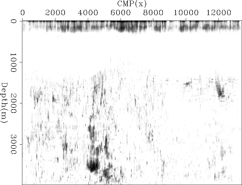
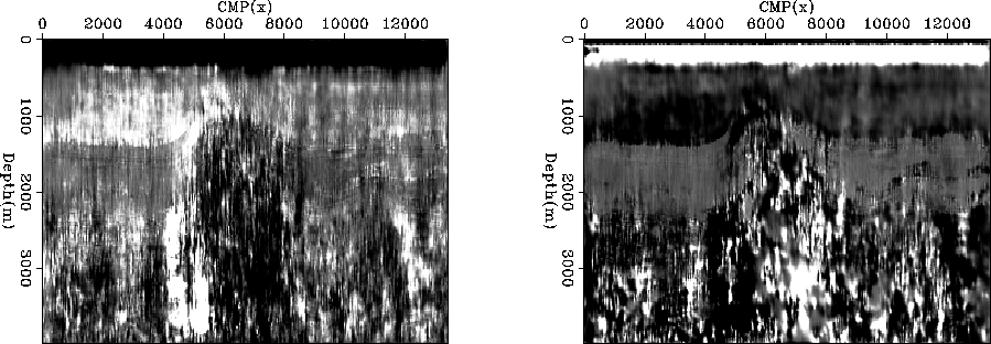
Figure ![[*]](http://sepwww.stanford.edu/latex2html/cross_ref_motif.gif) shows the result of stacking the absolute value of the
residual over
the offset plane. Areas of high amplitude represent areas where a single
parameter did not accurately describe
shows the result of stacking the absolute value of the
residual over
the offset plane. Areas of high amplitude represent areas where a single
parameter did not accurately describe  .
.
data
Figure 1 The left panel shows three cross-sections of
the migrated image (depth, inline, angle). The right panel shows
the time shifts calculated from the volume.


 rho1
rho1
Figure 2 The result of inverting for the moveout
parameter  from the time shifts shown in the
right panel of Figure
 ![[*]](http://sepwww.stanford.edu/latex2html/cross_ref_motif.gif) .
.


 resid1
Figure 3 The spatial error fitting error associated
with the time shifts shown in Figure ![[*]](http://sepwww.stanford.edu/latex2html/cross_ref_motif.gif) and the moveout parameter
shown in Figure
and the moveout parameter
shown in Figure ![[*]](http://sepwww.stanford.edu/latex2html/cross_ref_motif.gif) .
.


Rather than solving for a single moveout parameter at each location,
we can solve for multiple moveout parameters simultaneously. To test this
approach I introduced a new operator  that estimates
the moveout parameter
  by searching
for higher order moveout anomalies. For
  I chose an arbitrary moveout function,
|  |
(10) |
that attempts to see if a higher polynomial of the same form as  to
help to describe the moveout. The optimization
goal of equation (
 ) becomes
|  |
(11) |
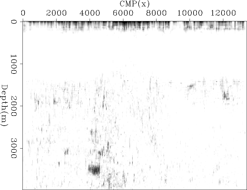
Figure ![[*]](http://sepwww.stanford.edu/latex2html/cross_ref_motif.gif) shows the resulting
shows the resulting  (left) and
  (right)
fields. Note how similar the
  field is to the one in Figure
 ![[*]](http://sepwww.stanford.edu/latex2html/cross_ref_motif.gif) ,
indicating that a two-stage estimation approach would have yielded a similar result. Figure
,
indicating that a two-stage estimation approach would have yielded a similar result. Figure ![[*]](http://sepwww.stanford.edu/latex2html/cross_ref_motif.gif) shows the resulting residual. Note the decrease in some areas compared to Figure
shows the resulting residual. Note the decrease in some areas compared to Figure ![[*]](http://sepwww.stanford.edu/latex2html/cross_ref_motif.gif) ,
but still showing areas where the moveout is significantly more complex.
rho2
,
but still showing areas where the moveout is significantly more complex.
rho2
Figure 4 The result of inverting for both  (left panel) and
  (right
panel). Note the similarity to the single parameter estimation shown in Figure
 ![[*]](http://sepwww.stanford.edu/latex2html/cross_ref_motif.gif) .
.


resid2
Figure 5 The fitting error associated with the two parameter fitting shown
in Figure ![[*]](http://sepwww.stanford.edu/latex2html/cross_ref_motif.gif) . .
|
|  |


The methodology of this section assumed that the  field was accurate. The non-linear
nature means this assumption is problematic, particularly when we are far from the correct solution.
In the context of the moveout problem, this means we are far from flat the defacto starting guess.


Next: Limiting flattening model space
Up: R. Clapp: Moveout analysis
Previous: Flattening Review
Stanford Exploration Project
5/6/2007
![]() field
that is function of depth z, offset h, and CRP
field
that is function of depth z, offset h, and CRP ![]() . As a first test
we want to estimate moveout of a volume migrated using downward continuation
migration. Biondi and Symes (2003) demonstrated that residual moveout
. As a first test
we want to estimate moveout of a volume migrated using downward continuation
migration. Biondi and Symes (2003) demonstrated that residual moveout ![]() can be approximated (assuming zero geologic dip)
as a function of angle
can be approximated (assuming zero geologic dip)
as a function of angle ![]() and depth z through
and depth z through
![[*]](http://sepwww.stanford.edu/latex2html/cross_ref_motif.gif) displays two cross-sections of the migrated
data (left) and the
displays two cross-sections of the migrated
data (left) and the ![]() field (right) calculated from the volume.
A moveout field
field (right) calculated from the volume.
A moveout field ![]() is then calculated from the
is then calculated from the
![]() field using a conjugate gradient algorithm to minimize
equation 9. Figure
field using a conjugate gradient algorithm to minimize
equation 9. Figure ![[*]](http://sepwww.stanford.edu/latex2html/cross_ref_motif.gif) shows the resulting
moveout field. The inversion approach has an additional advantage,
it easy to assess where the moveout parameterization effectively
described the time shifts and where it failed.
Figure
shows the resulting
moveout field. The inversion approach has an additional advantage,
it easy to assess where the moveout parameterization effectively
described the time shifts and where it failed.
Figure ![[*]](http://sepwww.stanford.edu/latex2html/cross_ref_motif.gif) shows the result of stacking the absolute value of the
residual over
the offset plane. Areas of high amplitude represent areas where a single
parameter did not accurately describe
shows the result of stacking the absolute value of the
residual over
the offset plane. Areas of high amplitude represent areas where a single
parameter did not accurately describe ![]() .
.
![[*]](http://sepwww.stanford.edu/latex2html/cross_ref_motif.gif) .
.
![[*]](http://sepwww.stanford.edu/latex2html/cross_ref_motif.gif) and the moveout parameter
shown in Figure
and the moveout parameter
shown in Figure ![[*]](http://sepwww.stanford.edu/latex2html/cross_ref_motif.gif) .
.
![]() that estimates
the moveout parameter
that estimates
the moveout parameter ![]() by searching
for higher order moveout anomalies. For
by searching
for higher order moveout anomalies. For ![]() I chose an arbitrary moveout function,
I chose an arbitrary moveout function,
![[*]](http://sepwww.stanford.edu/latex2html/cross_ref_motif.gif) shows the resulting
shows the resulting ![[*]](http://sepwww.stanford.edu/latex2html/cross_ref_motif.gif) ,
indicating that a two-stage estimation approach would have yielded a similar result. Figure
,
indicating that a two-stage estimation approach would have yielded a similar result. Figure ![[*]](http://sepwww.stanford.edu/latex2html/cross_ref_motif.gif) shows the resulting residual. Note the decrease in some areas compared to Figure
shows the resulting residual. Note the decrease in some areas compared to Figure ![[*]](http://sepwww.stanford.edu/latex2html/cross_ref_motif.gif) ,
but still showing areas where the moveout is significantly more complex.
,
but still showing areas where the moveout is significantly more complex.
![[*]](http://sepwww.stanford.edu/latex2html/cross_ref_motif.gif) .
.
![[*]](http://sepwww.stanford.edu/latex2html/cross_ref_motif.gif) .
.

![]() field was accurate. The non-linear
nature means this assumption is problematic, particularly when we are far from the correct solution.
In the context of the moveout problem, this means we are far from flat the defacto starting guess.
field was accurate. The non-linear
nature means this assumption is problematic, particularly when we are far from the correct solution.
In the context of the moveout problem, this means we are far from flat the defacto starting guess.