

Next: Conclusions
Up: R. Clapp: Moveout analysis
Previous: Post-flattening inversion
The two-stage approach of the last section is only applicable
when the  estimation is able to fully
describe the moveout in the gather. When it cannot, another approach
must be found. The left panel of Figure
 ![[*]](http://sepwww.stanford.edu/latex2html/cross_ref_motif.gif) is a synthetic CMP gather
created by bandpassing random numbers, and then spraying them
out with adjoint of NMO. The right panel of Figure
is a synthetic CMP gather
created by bandpassing random numbers, and then spraying them
out with adjoint of NMO. The right panel of Figure ![[*]](http://sepwww.stanford.edu/latex2html/cross_ref_motif.gif) shows the result
of estimating time shifts (7 Gauss-Newton steps) and then
applying those time shifts to flatten the data. Note that the flattening
approach has failed in several areas.
syn
shows the result
of estimating time shifts (7 Gauss-Newton steps) and then
applying those time shifts to flatten the data. Note that the flattening
approach has failed in several areas.
syn
Figure 6 The left panel is a synthetic CMP gather.
The right panel shows the result of flattening the CMP gather using the standard
approach. Note the waviness of several reflectors due to the the non-linear nature
of the flattening technique.


Estimation of the time shifts is problematic
because the problem is inherently non-linear. One successful
strategy is to try to start with an initial guess that is as close as possible to the correct
solution. Another is to limit the model space to feasible
candidates. In this simple case we know that the moveout is
governed by the NMO equation. We can linearize the NMO equation that
relates time shifts  , zero offset time t0, offset h, and slowness s through
|  |
(12) |
around
our initial slowness  . We obtain an equation,
|  |
(13) |
that relates  to
to  . The implied operator
  then helps
to form the linearized optimization equation,
|  |
(14) |
In practice we need to add an additional weighting operator  which
accounts for areas effected wavelet stretch and for reflections that exist
at zero offset, but not at larger offsets. As a result we must
use a space-domain conjugate gradient scheme
|  |
(15) |
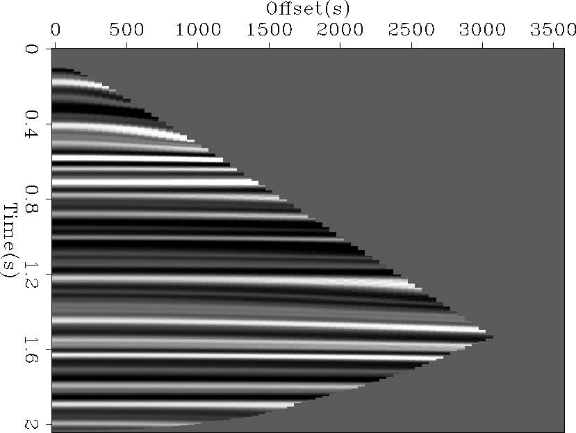
Figure ![[*]](http://sepwww.stanford.edu/latex2html/cross_ref_motif.gif) shows the flattened CMP gather using the slowness model
space description. While not perfect, the result is significantly flatter
than the alternative approach (right panel of Figure
shows the flattened CMP gather using the slowness model
space description. While not perfect, the result is significantly flatter
than the alternative approach (right panel of Figure ![[*]](http://sepwww.stanford.edu/latex2html/cross_ref_motif.gif) ).
).
cmp
Figure 7 The flattened CMP gather using a Gauss-Newton scheme
with the model space limited to hyperbolic moveout. The result is much flatter
than the standard parameterization scheme show in the right panel of Figure ![[*]](http://sepwww.stanford.edu/latex2html/cross_ref_motif.gif) . .
|
|  |


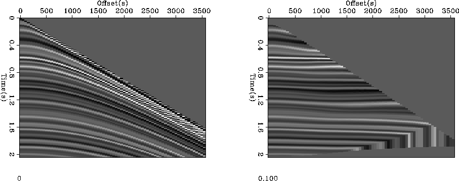
Figure ![[*]](http://sepwww.stanford.edu/latex2html/cross_ref_motif.gif) shows the result of applying both techniques to
a CMP gather from the same North Sea dataset used in the previous
section. The left panel is the raw gather, the center panel uses the
conventional technique, and the right panel limits the moveout description
to a single hyperbolic parameter. Note how both approaches fail at
early times but the hyperbolic description provides noticably better result.
shows the result of applying both techniques to
a CMP gather from the same North Sea dataset used in the previous
section. The left panel is the raw gather, the center panel uses the
conventional technique, and the right panel limits the moveout description
to a single hyperbolic parameter. Note how both approaches fail at
early times but the hyperbolic description provides noticably better result.
elf
Figure 8 A CMP gather from the North Sea. The left panel shows
the original gather. The center panel shows the result of using a standard
parameterization for flattening. The right panel is the result using a
hperbolic parameterization.


Next: Conclusions
Up: R. Clapp: Moveout analysis
Previous: Post-flattening inversion
Stanford Exploration Project
5/6/2007

![[*]](http://sepwww.stanford.edu/latex2html/cross_ref_motif.gif) is a synthetic CMP gather
created by bandpassing random numbers, and then spraying them
out with adjoint of NMO. The right panel of Figure
is a synthetic CMP gather
created by bandpassing random numbers, and then spraying them
out with adjoint of NMO. The right panel of Figure ![[*]](http://sepwww.stanford.edu/latex2html/cross_ref_motif.gif) shows the result
of estimating time shifts (7 Gauss-Newton steps) and then
applying those time shifts to flatten the data. Note that the flattening
approach has failed in several areas.
shows the result
of estimating time shifts (7 Gauss-Newton steps) and then
applying those time shifts to flatten the data. Note that the flattening
approach has failed in several areas.

![]() , zero offset time t0, offset h, and slowness s through
, zero offset time t0, offset h, and slowness s through

![[*]](http://sepwww.stanford.edu/latex2html/cross_ref_motif.gif) shows the flattened CMP gather using the slowness model
space description. While not perfect, the result is significantly flatter
than the alternative approach (right panel of Figure
shows the flattened CMP gather using the slowness model
space description. While not perfect, the result is significantly flatter
than the alternative approach (right panel of Figure ![[*]](http://sepwww.stanford.edu/latex2html/cross_ref_motif.gif) ).
).
![[*]](http://sepwww.stanford.edu/latex2html/cross_ref_motif.gif) .
.

![[*]](http://sepwww.stanford.edu/latex2html/cross_ref_motif.gif) shows the result of applying both techniques to
a CMP gather from the same North Sea dataset used in the previous
section. The left panel is the raw gather, the center panel uses the
conventional technique, and the right panel limits the moveout description
to a single hyperbolic parameter. Note how both approaches fail at
early times but the hyperbolic description provides noticably better result.
shows the result of applying both techniques to
a CMP gather from the same North Sea dataset used in the previous
section. The left panel is the raw gather, the center panel uses the
conventional technique, and the right panel limits the moveout description
to a single hyperbolic parameter. Note how both approaches fail at
early times but the hyperbolic description provides noticably better result.
