


Volume ![]() will have a global mean, which we take to be the sample mean
will have a global mean, which we take to be the sample mean
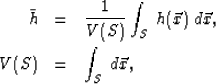 |
(1) | |
| (2) |
Since volume ![]() maps to
maps to ![]() , with V(S) defined by Eq. 2, the DC component of
, with V(S) defined by Eq. 2, the DC component of ![]() corresponding to the gray background is mostly removed. Then,
corresponding to the gray background is mostly removed. Then, ![]() . The algorithm adds the primarily low-frequency
. The algorithm adds the primarily low-frequency ![]() to the almost DC-less
to the almost DC-less ![]() to synthesize
to synthesize ![]() .
.
In practice, a scaled ![]() is added to
is added to ![]() to avoid significant alteration of local means when going from
to avoid significant alteration of local means when going from ![]() to
to ![]() . The exact value of alpha depends on the relative signal levels in
. The exact value of alpha depends on the relative signal levels in ![]() and
and ![]() . Relating back to the framework in Fig. 3, the upper branch's extraction of high-frequency components from
. Relating back to the framework in Fig. 3, the upper branch's extraction of high-frequency components from ![]() and scaling are contained in the term
and scaling are contained in the term ![]() . The lower branch's behavior is simpler: all frequency components are extracted from
. The lower branch's behavior is simpler: all frequency components are extracted from ![]() and the scaling factor is unity.
and the scaling factor is unity.
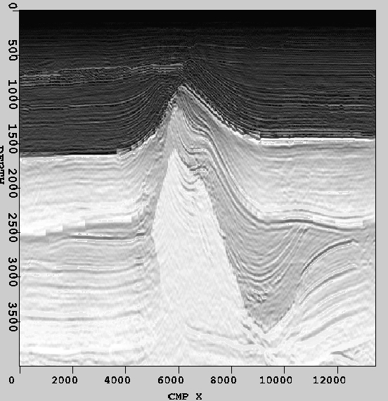
The synthesized result of the slices from Fig. 1 is shown in Fig. 4. It can be seen that the first algorithm performs well in presenting the fine details of ![]() . Because we avoided significant alteration of the local means of
. Because we avoided significant alteration of the local means of ![]() through the scaling factor
through the scaling factor ![]() , the textural smoothness and regional boundaries of
, the textural smoothness and regional boundaries of ![]() are well preserved.
are well preserved.
 |
