Data-fusion using deviation-dependent weighting

Instead of adjusting the intensities of $l(\vec{x})$, the second algorithm synthesizes a new volume from a convex combination of the source volumes $h(\vec{x})$ and $l(\vec{x})$. The relative levels of contribution from $h(\vec{x})$ and $l(\vec{x})$ are determined by how much $h(\vec{x})$ deviates from $\bar{h}$, where $\bar{h}$ is defined by Eq. 1 and is the intensity of the gray background in $h(\vec{x})$. Specifically, we form

$$\begin{eqnarray} m_2(\vec{x}) &=& \beta(\vec{x}) \cdot h(\vec{x}) + (1-\beta(\ve... ...h}\vert} {max\{\vert h(\vec{x})-\bar{h}\vert : \vec{x} \in S \}} ,\end{eqnarray}$$ (3) (4)

where S is the data space. As can be seen from Eq. 4, $\beta(\vec{x})$ is spatially-varying weighting factor between 0 and 1. As $\beta(\vec{x}) \rightarrow 1$, corresponding to large deviations from $\bar{h}$, $m_2(\vec{x}) \rightarrow h(\vec{x})$. For $\beta(\vec{x}) \rightarrow 0$, corresponding to small deviations from $\bar{h}$, $m_2(\vec{x}) \rightarrow l(\vec{x})$. The result m₂(x) leans more towards $h(\vec{x})$ where local structures appear and more towards $l(\vec{x})$ otherwise. Another advantage of using the convex combination in Eq. 2 is that if $\beta(\vec{x})$ varies smoothly in space, then the synthesized volume $m_2(\vec{x})$ will also vary smoothly in space.

Here, in terms of the framework in Fig. 3, the upper branch's extraction of high-frequency components from $h(\vec{x})$ and scaling depicted are contained in the term $\beta(\vec{x}) \cdot h(\vec{x})$. Similarly, the lower branch's extraction of low-frequency components from $l(\vec{x})$ and scaling are contained in the term $(1-\beta(\vec{x})) \cdot l(\vec{x})$.

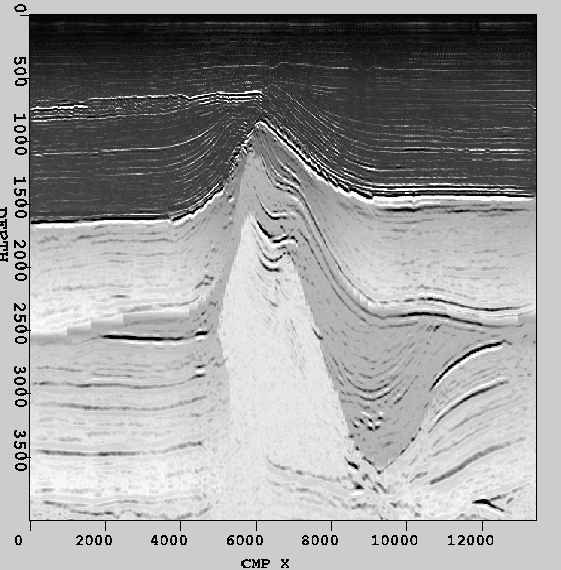
When combining the slices from Fig. 1, we obtained the synthesized result shown in Fig. 5. The advantage of the second algorithm is that it synthesizes the local structures from $h(\vec{x})$ in the new volume more accurately than does the first algorithm, but this is done at the expense of sacrificing a small amount of textural smoothness inherited from $l(\vec{x})$. Again, the local means from $l(\vec{x})$ are well preserved.

 

chen-velview-merge2
Figure 5 Result using the second data-fusion algorithm.