![[*]](http://sepwww.stanford.edu/latex2html/cross_ref_motif.gif) .
.
Iterative least-squares inversion is a computationally expensive way to equalize amplitudes in areas of poor illumination. A less expensive method to equalize amplitudes is simple weighting in the model space. Model space weighting operators can be applied to an image after it has been produced by a migration operator. () suggested using the velocity model and a downward-continuation operator to give us an appropriate weighting operator that will compensate for illumination.
In this section, I will first review the method proposed by () for the construction of a model space weighting operator. I will then apply this weighting operator to a complex synthetic model with clear illumination problems. Finally, I will compare the model space weighted results with the more expensive preconditioned inversion method I have introduced in this chapter.
() described a simple a posteriori diagonal weighting operator 60#60.To approximate 60#60, we begin by formulating our imaging operation as
| 61#61 | (27) |
The question now is how to get 60#60.() showed that by applying a forward operator and its adjoint to a reference model, we will get a weighting function with the correct physical units. () took it a step further to show that for illumination, we can find the approximate weighting function in this manner:
| 62#62 | (28) |
Here 63#63 is the chosen reference model, 40#40is a damping parameter related to the signal-to-noise ratio, and the <> indicate that we take the smoothed analytic signal envelopes. 40#40 ensures that we will not be dividing by zero.
In order to examine this weighting operator, I chose to work with the
subset of the Sigsbee2A dataset I have shown before. This dataset has a salt
body with strong shadow zones beneath its edges. The velocity model can
be seen in Figure ![[*]](http://sepwww.stanford.edu/latex2html/cross_ref_motif.gif) .
.
 |
I chose to use flat layers as the reference model, as suggested by
(). I modeled the data that would
be produced from these flat layers with the adjoint of the migration scheme
described in the previous subsection, using the velocity model from
Figure ![[*]](http://sepwww.stanford.edu/latex2html/cross_ref_motif.gif) . I then migrated that data to get the weighting
operator defined in equation (
. I then migrated that data to get the weighting
operator defined in equation (![[*]](http://sepwww.stanford.edu/latex2html/cross_ref_motif.gif) ). Figure
). Figure ![[*]](http://sepwww.stanford.edu/latex2html/cross_ref_motif.gif) shows
this weighting operator.
shows
this weighting operator.
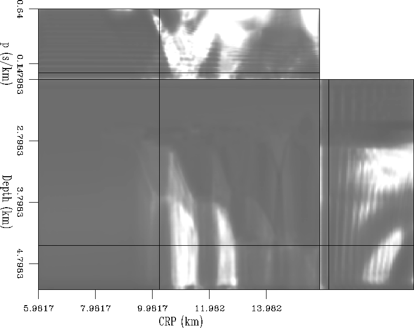
The weighting operator in Figure ![[*]](http://sepwww.stanford.edu/latex2html/cross_ref_motif.gif) is displayed as a flattened
cube. The front of the cube shows a common ray parameter slice in which
the high values of the weighting operator can be seen in the shadow zones. The
top of the cube is shown above the common ray parameter slice and shows a
depth slice. In this depth slice, we can see that the weighting operator
indicates that the subsalt illumination along CRPs is becoming worse with
larger ray parameters. The side of the cube shows a ray parameter gather
taken from a CRP at the salt edge. This view shows how illumination
varies along ray parameter and with depth. It also shows some vertical
striping that I believe is caused by the way I took the smoothed analytic
signal envelope. We must keep this in mind as we apply this weighting function
to the image.
is displayed as a flattened
cube. The front of the cube shows a common ray parameter slice in which
the high values of the weighting operator can be seen in the shadow zones. The
top of the cube is shown above the common ray parameter slice and shows a
depth slice. In this depth slice, we can see that the weighting operator
indicates that the subsalt illumination along CRPs is becoming worse with
larger ray parameters. The side of the cube shows a ray parameter gather
taken from a CRP at the salt edge. This view shows how illumination
varies along ray parameter and with depth. It also shows some vertical
striping that I believe is caused by the way I took the smoothed analytic
signal envelope. We must keep this in mind as we apply this weighting function
to the image.
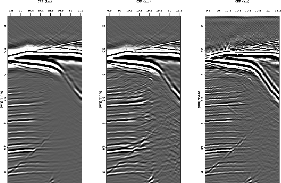
Figure ![[*]](http://sepwww.stanford.edu/latex2html/cross_ref_motif.gif) shows
an enlarged view of the stacks in the area at the salt edge for the
downward-continuation migration (left panel),
the model space weighted result (center), and the preconditioned inversion
result (right panel). In the migration result, the noise in the shadow
zones is not very strong, but the upswinging artifacts (particularly below
a depth of 4.25 kilometers) can easily cause misinterpretation. The model
space weighted result has extended the
reflectors farther under the salt than the migration result, but it also
has increased noise under the salt and strengthened the upswinging
artifacts. The inversion result has done a better job of
extending the reflectors beneath the salt and has fewer artifacts than
either of the other results. The inversion result has eliminated the
upswinging artifacts seen in both the migration and the model space
weighted result. However, the inversion result has a
computational cost approximately seven
times
shows
an enlarged view of the stacks in the area at the salt edge for the
downward-continuation migration (left panel),
the model space weighted result (center), and the preconditioned inversion
result (right panel). In the migration result, the noise in the shadow
zones is not very strong, but the upswinging artifacts (particularly below
a depth of 4.25 kilometers) can easily cause misinterpretation. The model
space weighted result has extended the
reflectors farther under the salt than the migration result, but it also
has increased noise under the salt and strengthened the upswinging
artifacts. The inversion result has done a better job of
extending the reflectors beneath the salt and has fewer artifacts than
either of the other results. The inversion result has eliminated the
upswinging artifacts seen in both the migration and the model space
weighted result. However, the inversion result has a
computational cost approximately seven
times ![[*]](http://sepwww.stanford.edu/latex2html/foot_motif.gif) greater than the weighted result.
greater than the weighted result.
 |
To summarize, although the model space weighting operator does help improve the amplitudes in poorly illuminated areas of seismic images, it does not do as good a job as the least-squares inversion. This is largely due to the fact that the weighting operator increases the amplitude of the noise as well as that of the signal. Regularized least-squares inversion does a better job compensating for poor illumination in areas with low signal-to-noise ratios and helps to reduce artifacts.