Accommodating the model space regularization in the data space

Although 57#57 and 58#58 are useful for obtaining a clean inversion result, 56#56 is vital in the regularized inversion process. The regularization of the model compensates for poor illumination, some of which is caused by energy leaving the extents of the survey. Since the regularization helps to recover this energy, we need to be able to map it into the data space when the forward operation 29#29 is performed within the conjugate-gradient iteration. This means that we need to pad the offset axis in the data space. However, we don't want to include this energy in the residual space, so we use the weighting operator 56#56 to mask it out.

In addition to the ``recovered'' data along the offset axis, regularization will also introduce frequencies that were not in the recorded data. This occurs because the regularization may be designed in a way that mixes the images corresponding to different aperture angles. When this occurs, it has the effect of equalizing the vertical wavenumber content across the angle axis. The shorter wavelengths are spread from the near-vertical incidence images toward the wide-aperture angle images and the longer wavelengths are spread from far angles to near angles. 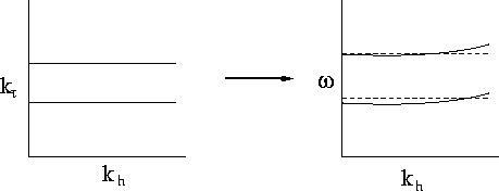A sketch of how this occurs can be seen in Figure . The plane on the left is the model space where the regularization is acting. For the purpose of this explanation, assume that the regularization spreads energy fully between the horizontal lines. When this is mapped to the data space (right plane), those bounding lines curve as shown. The dashed lines show the frequency range of the original data. As with the offset axis, the data space must be padded along the frequency axis to allow the "recovery" of the frequencies as well.

 

freqpad
Figure 12 Constant velocity example of ``lost'' frequencies. Left: model space where regularization spreads energy throughout the region bounded by the two horizontal lines. Right: data space where the two bounding lines now curve upward. The dashed lines indicate the frequency range of the original data.