

Next: Multiple subtraction
Up: Multiple attenuation: A 3-D
Previous: Shot interpolation of the
Having interpolated the shots to a 25 m grid makes the multiple
prediction more accurate. Figure ![[*]](http://sepwww.stanford.edu/latex2html/cross_ref_motif.gif) shows a
comparison for one offset of the input data and the predicted multiples
with and without sparse interpolation. The predicted multiples in
Figures
shows a
comparison for one offset of the input data and the predicted multiples
with and without sparse interpolation. The predicted multiples in
Figures ![[*]](http://sepwww.stanford.edu/latex2html/cross_ref_motif.gif) b and
b and ![[*]](http://sepwww.stanford.edu/latex2html/cross_ref_motif.gif) c look
almost identical to the true multiples in Figure
c look
almost identical to the true multiples in Figure
![[*]](http://sepwww.stanford.edu/latex2html/cross_ref_motif.gif) a. Some artifacts, shown as A in Figure
a. Some artifacts, shown as A in Figure
![[*]](http://sepwww.stanford.edu/latex2html/cross_ref_motif.gif) c, are nevertheless present
in the multiple model obtained from the interpolated data without
regularization. These artifacts come from the convolution
of the noise visible in Figure
c, are nevertheless present
in the multiple model obtained from the interpolated data without
regularization. These artifacts come from the convolution
of the noise visible in Figure ![[*]](http://sepwww.stanford.edu/latex2html/cross_ref_motif.gif) b before the
water-bottom reflection with coherent
energy. Some of them could be attenuated by applying a mute on the
interpolated shot gathers.
b before the
water-bottom reflection with coherent
energy. Some of them could be attenuated by applying a mute on the
interpolated shot gathers.
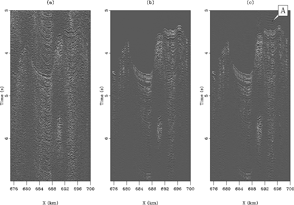
window1-recons
Figure 9 Close-ups of common-offset
gathers in the vicinity of
first-order multiples at 250 m offset for (a) the input data, (b) the predicted
multiples with the sparseness constraint, and (c) the predicted
multiples without regularization. traint, and (c) the predicted
multiples without regularization. The horizontal axis represents the
midpoint position. Arrow A points to artifacts in the
multiple prediction that are caused by interpolation errors.


The multiple model looks relatively accurate for the whole
section. However, some important discrepancies exist between the true and
modeled multiples in some places. For instance, Figure
![[*]](http://sepwww.stanford.edu/latex2html/cross_ref_motif.gif) displays the multiple prediction results in
an area where the model does not match the observed multiples very
well. In Figure
displays the multiple prediction results in
an area where the model does not match the observed multiples very
well. In Figure ![[*]](http://sepwww.stanford.edu/latex2html/cross_ref_motif.gif) b, the water-bottom multiple
(shown as 1) is clearly modeled better with the interpolated data
with sparseness constraint than in Figure
b, the water-bottom multiple
(shown as 1) is clearly modeled better with the interpolated data
with sparseness constraint than in Figure ![[*]](http://sepwww.stanford.edu/latex2html/cross_ref_motif.gif) c
without regularization.
The two circles in Figure
c
without regularization.
The two circles in Figure ![[*]](http://sepwww.stanford.edu/latex2html/cross_ref_motif.gif) b and
b and
![[*]](http://sepwww.stanford.edu/latex2html/cross_ref_motif.gif) c highlight aliasing artifacts that are also
visible in Figures
c highlight aliasing artifacts that are also
visible in Figures ![[*]](http://sepwww.stanford.edu/latex2html/cross_ref_motif.gif) b and
b and
![[*]](http://sepwww.stanford.edu/latex2html/cross_ref_motif.gif) c. These artifacts would disappear by having
a smaller sampling of both shot and offset axes. Therefore, these
aliasing artifacts are stronger when no Cauchy regularization
is applied for the interpolation.
c. These artifacts would disappear by having
a smaller sampling of both shot and offset axes. Therefore, these
aliasing artifacts are stronger when no Cauchy regularization
is applied for the interpolation.
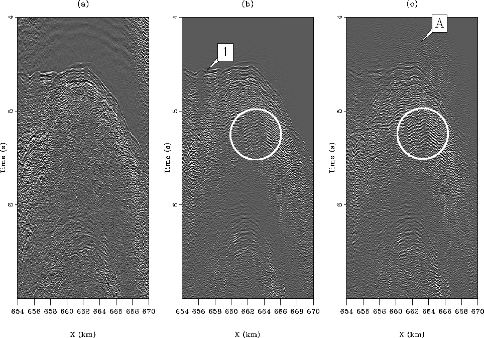
window2-recons
Figure 10 Close-ups of common-offset
gathers in the vicinity of first-order multiples at 4.425 km offset
for (a) the input data, (b) the predicted
multiples with the sparseness constraint, and (c) the predicted
multiples without regularization. The horizontal axis represents the
midpoint position. 1 points to the water-bottom
multiple that is better modeled when the Cauchy regularization is
used for interpolation. Arrow A points to artifacts similar to those in
Figure ![[*]](http://sepwww.stanford.edu/latex2html/cross_ref_motif.gif) c. The two circles point to aliasing
artifacts created during the multiple prediction.
c. The two circles point to aliasing
artifacts created during the multiple prediction.


Looking now at shot gathers in Figure ![[*]](http://sepwww.stanford.edu/latex2html/cross_ref_motif.gif) , it
appears that the modeling of multiples worked well for the main
reflection events. Energetic diffracted multiples are almost totally absent in the
predictions of Figures
, it
appears that the modeling of multiples worked well for the main
reflection events. Energetic diffracted multiples are almost totally absent in the
predictions of Figures ![[*]](http://sepwww.stanford.edu/latex2html/cross_ref_motif.gif) b and
b and
![[*]](http://sepwww.stanford.edu/latex2html/cross_ref_motif.gif) c, however. Diffracted multiples are generally
more difficult to model because they require a very dense surface
coverage of sources and receivers in order to recover all the dips
(Figure
c, however. Diffracted multiples are generally
more difficult to model because they require a very dense surface
coverage of sources and receivers in order to recover all the dips
(Figure ![[*]](http://sepwww.stanford.edu/latex2html/cross_ref_motif.gif) ). This effect is amplified in 3-D.
Approximating the sail line as a
continuous 2-D survey and ignoring 3-D effects lead to large errors
in the model of diffracted multiples.
). This effect is amplified in 3-D.
Approximating the sail line as a
continuous 2-D survey and ignoring 3-D effects lead to large errors
in the model of diffracted multiples.
window3-recons
Figure 11 Shot gather at 661.65 km for
(a) the input data, (b) the predicted
multiples with the sparseness constraint, and (c) the predicted
multiples without regularization. D points to diffracted multiples that
are not properly modeled in either (b) or (c). AA points to aliasing
artifacts that create the fictitious events in the circles of Figure ![[*]](http://sepwww.stanford.edu/latex2html/cross_ref_motif.gif) .
.


The estimation of a multiple model with a 2-D prediction scheme for
3-D field data, although being accurate in most places, suffers from
kinematic and amplitude errors. For some events, e.g., diffracted
multiples, the modeling fails completely. In addition, the shot
interpolation technique needs to be chosen carefully to minimize its
impact on the final multiple model. Here, the radon-based approach
with a sparseness constraint yields the best multiple model.
Given this imperfect model, it is now the goal of the subtraction to come up with the best
estimated primaries. In the next section, multiple attenuation results are
presented with a pattern-based and adaptive subtraction technique.


Next: Multiple subtraction
Up: Multiple attenuation: A 3-D
Previous: Shot interpolation of the
Stanford Exploration Project
5/5/2005
![[*]](http://sepwww.stanford.edu/latex2html/cross_ref_motif.gif) shows a
comparison for one offset of the input data and the predicted multiples
with and without sparse interpolation. The predicted multiples in
Figures
shows a
comparison for one offset of the input data and the predicted multiples
with and without sparse interpolation. The predicted multiples in
Figures ![[*]](http://sepwww.stanford.edu/latex2html/cross_ref_motif.gif) b and
b and ![[*]](http://sepwww.stanford.edu/latex2html/cross_ref_motif.gif) c look
almost identical to the true multiples in Figure
c look
almost identical to the true multiples in Figure
![[*]](http://sepwww.stanford.edu/latex2html/cross_ref_motif.gif) a. Some artifacts, shown as A in Figure
a. Some artifacts, shown as A in Figure
![[*]](http://sepwww.stanford.edu/latex2html/cross_ref_motif.gif) c, are nevertheless present
in the multiple model obtained from the interpolated data without
regularization. These artifacts come from the convolution
of the noise visible in Figure
c, are nevertheless present
in the multiple model obtained from the interpolated data without
regularization. These artifacts come from the convolution
of the noise visible in Figure ![[*]](http://sepwww.stanford.edu/latex2html/cross_ref_motif.gif) b before the
water-bottom reflection with coherent
energy. Some of them could be attenuated by applying a mute on the
interpolated shot gathers.
b before the
water-bottom reflection with coherent
energy. Some of them could be attenuated by applying a mute on the
interpolated shot gathers.


