

Next: Multiple prediction results
Up: Interpolation
Previous: Theory
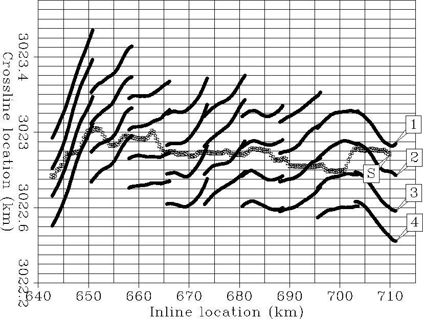
Figure ![[*]](http://sepwww.stanford.edu/latex2html/cross_ref_motif.gif) shows the acquisition
geometry for one particular sail line. The first streamer (shown as 1)
is extracted and used for this field data example.
The ship is moving from right to left. Surface currents
generate strong cable feathering around 642 km in the inline
direction. The receiver positions are displayed for nine shots
only every eight kilometers in Figure
shows the acquisition
geometry for one particular sail line. The first streamer (shown as 1)
is extracted and used for this field data example.
The ship is moving from right to left. Surface currents
generate strong cable feathering around 642 km in the inline
direction. The receiver positions are displayed for nine shots
only every eight kilometers in Figure ![[*]](http://sepwww.stanford.edu/latex2html/cross_ref_motif.gif) .
.
shotline-10
Figure 2 Acquisition geometry for
one sail line. S points to the locations of one source going from
710 km to 642 km. 1,2,3 and 4 points to the receiver lines
for the four different streamers.
The receiver locations (black lines) are shown for nine shots
for the entire sail line. The data corresponding to streamer 1
are processed in this Chapter.

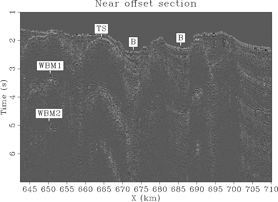
A near offset section for streamer 1 in Figure ![[*]](http://sepwww.stanford.edu/latex2html/cross_ref_motif.gif) is shown in Figure
is shown in Figure ![[*]](http://sepwww.stanford.edu/latex2html/cross_ref_motif.gif) . Salt intrusions make the S/N ratio very low
below three seconds. Two orders of surface-related multiples (WBM1 and
WBM2) are present in the data. The trace spacing is 75 m. The goal is
to interpolate the shots every 25 m and to recover the near
offset information before 2-D SRMP.
. Salt intrusions make the S/N ratio very low
below three seconds. Two orders of surface-related multiples (WBM1 and
WBM2) are present in the data. The trace spacing is 75 m. The goal is
to interpolate the shots every 25 m and to recover the near
offset information before 2-D SRMP.
nearoffset
Figure 3 Near offset section
(h=250 m) from streamer 1 in Figure ![[*]](http://sepwww.stanford.edu/latex2html/cross_ref_motif.gif) . TS points
to top of salt reflections. B points to sedimentary basins. WBM1 points
to a first-order surface related multiple and WBM2 points to a
second-order surface related multiple. The S/N ratio is
extremely low below the salt.
. TS points
to top of salt reflections. B points to sedimentary basins. WBM1 points
to a first-order surface related multiple and WBM2 points to a
second-order surface related multiple. The S/N ratio is
extremely low below the salt.


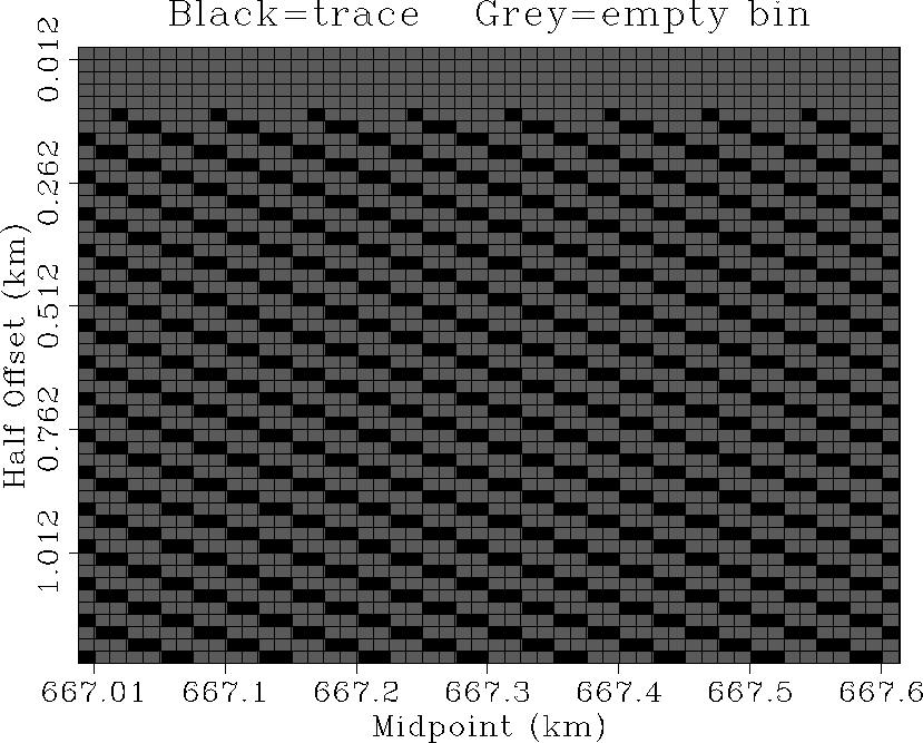
The shot gathers are first sorted into CMP gathers. The binning
parameters are illustrated in Figure ![[*]](http://sepwww.stanford.edu/latex2html/cross_ref_motif.gif) . The bin size
is 25
. The bin size
is 25 12.5 m. The goal of the interpolation is to
fill-up the empty bins shown in Figure
 ![[*]](http://sepwww.stanford.edu/latex2html/cross_ref_motif.gif) . From the
CMP gathers, a masking operator
. From the
CMP gathers, a masking operator  is built. This masking
operator is set to zero where traces are missing and to one where
traces are present.
cmp-geo
Figure 4 Subset of the offset and CMP
distributions. The bin size is 12.5 m along the CMP axis
and 25 m along the offset axis. The CMP gathers are interpolated along
the offset axis to recover the missing shots and the near offset
information.


From the CMP gathers and the masking operator, a model  is
estimated by minimizing equations (
is
estimated by minimizing equations (![[*]](http://sepwww.stanford.edu/latex2html/cross_ref_motif.gif) ) and
(
) and
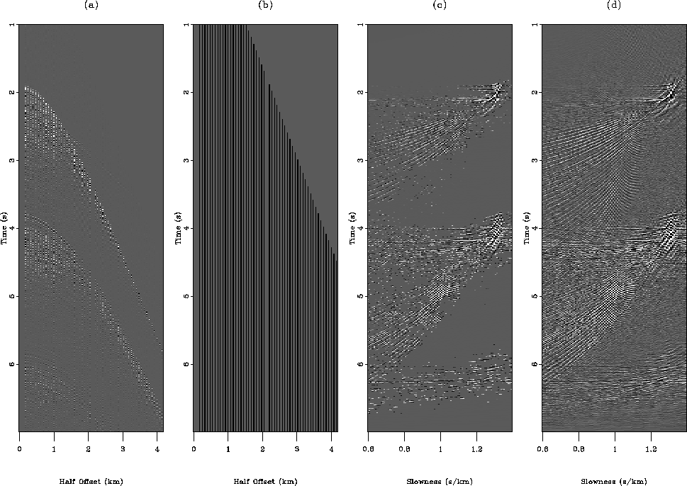
(![[*]](http://sepwww.stanford.edu/latex2html/cross_ref_motif.gif) ). Figures
). Figures ![[*]](http://sepwww.stanford.edu/latex2html/cross_ref_motif.gif) c and
c and ![[*]](http://sepwww.stanford.edu/latex2html/cross_ref_motif.gif) d show
d show  when the sparseness constraint is or is not applied, respectively.
Most of the aliasing artifacts caused by the missing traces in Figure
![[*]](http://sepwww.stanford.edu/latex2html/cross_ref_motif.gif) are well attenuated when the Cauchy regularization is
used. Note that the remaining artifacts in Figure
are well attenuated when the Cauchy regularization is
used. Note that the remaining artifacts in Figure ![[*]](http://sepwww.stanford.edu/latex2html/cross_ref_motif.gif) c could
be attenuated by increasing
c could
be attenuated by increasing  in equation
(
in equation
(![[*]](http://sepwww.stanford.edu/latex2html/cross_ref_motif.gif) ) with the possible effect of damaging some
useful signal, e.g., below 5 s in Figure
) with the possible effect of damaging some
useful signal, e.g., below 5 s in Figure ![[*]](http://sepwww.stanford.edu/latex2html/cross_ref_motif.gif) a.
a.
hrt
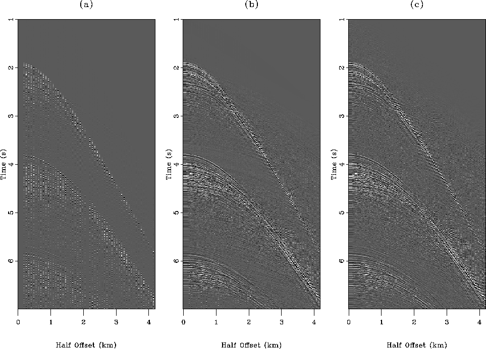
Figure 5 Illustration of the radon
transform for one CMP gather. (a) Input CMP gather showing strong
primaries around 2 s, first-order multiples near 4 s, and
second-order multiples near 6 s. (b) Masking
operator  . The black stripes are located at the known data
locations (Mi,i=1) while the rest of the mask is set to zero.
(c) Radon domain with Cauchy regularization,
i.e., equation (
. The black stripes are located at the known data
locations (Mi,i=1) while the rest of the mask is set to zero.
(c) Radon domain with Cauchy regularization,
i.e., equation (![[*]](http://sepwww.stanford.edu/latex2html/cross_ref_motif.gif) ). (d) Radon domain without
Cauchy regularization, i.e., equation (
). (d) Radon domain without
Cauchy regularization, i.e., equation (![[*]](http://sepwww.stanford.edu/latex2html/cross_ref_motif.gif) ).
).


Once  is estimated, the interpolated CMP gathers can be
created with equation (
is estimated, the interpolated CMP gathers can be
created with equation (![[*]](http://sepwww.stanford.edu/latex2html/cross_ref_motif.gif) ). Figure
). Figure ![[*]](http://sepwww.stanford.edu/latex2html/cross_ref_motif.gif) illustrates the interpolation result for one CMP gather. The
sparseness constraint (Figure
illustrates the interpolation result for one CMP gather. The
sparseness constraint (Figure ![[*]](http://sepwww.stanford.edu/latex2html/cross_ref_motif.gif) b)
gives a cleaner result and preserve the steep dips better than
the radon transform without regularization (Figure
b)
gives a cleaner result and preserve the steep dips better than
the radon transform without regularization (Figure
![[*]](http://sepwww.stanford.edu/latex2html/cross_ref_motif.gif) c). Note that the reconstructed traces are
less noisy than the known data and that adding some white
noise might be needed Gulunay (2003). Because the shots
are interpolated for multiple prediction only, no processing is applied
to correct for this defect.
c). Note that the reconstructed traces are
less noisy than the known data and that adding some white
noise might be needed Gulunay (2003). Because the shots
are interpolated for multiple prediction only, no processing is applied
to correct for this defect.
cmp-recons
Figure 6 (a) Input gather with missing
traces. (b) Reconstructed gather with the Cauchy regularization.
(c) Reconstructed gather without regularization.


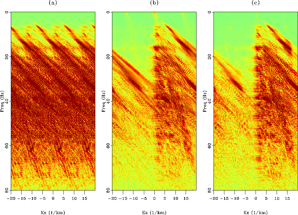
To better understand the effect of the Cauchy regularization on the
steep dips, Figures ![[*]](http://sepwww.stanford.edu/latex2html/cross_ref_motif.gif) a,
a, ![[*]](http://sepwww.stanford.edu/latex2html/cross_ref_motif.gif) b, and
b, and
![[*]](http://sepwww.stanford.edu/latex2html/cross_ref_motif.gif) c show the F-K spectra of the CMP gathers in Figure
c show the F-K spectra of the CMP gathers in Figure
![[*]](http://sepwww.stanford.edu/latex2html/cross_ref_motif.gif) for the
input data, the reconstructed data with sparseness constraint and the
reconstructed data without regularization, respectively. Most of the
steep dips are attenuated when no regularization is applied during the
inversion. This effect is clearly shown in the 15-25 Hz band where the
sparse interpolation shows some aliased energy for events going slower
than 1700 m/s (Figure
for the
input data, the reconstructed data with sparseness constraint and the
reconstructed data without regularization, respectively. Most of the
steep dips are attenuated when no regularization is applied during the
inversion. This effect is clearly shown in the 15-25 Hz band where the
sparse interpolation shows some aliased energy for events going slower
than 1700 m/s (Figure ![[*]](http://sepwww.stanford.edu/latex2html/cross_ref_motif.gif) b). The same events are
attenuated when no regularization is applied in Figure
b). The same events are
attenuated when no regularization is applied in Figure ![[*]](http://sepwww.stanford.edu/latex2html/cross_ref_motif.gif) c.
Therefore, inversion with Cauchy regularization is preferred
for data interpolation in the CMP domain.
Note that the aliased energy could be attenuated in the CMP domain
by sampling the offset axis on a thinner grid. However, because SRMP is
performed in the shot domain, it is difficult to anticipate the effects
of this aliasing on the multiple prediction result. In addition, by
resampling the CMP offset axis, more CMP gathers would be needed
to maintain a uniform grid in the shot domain for the multiple prediction.
This extra-requirement would increase the total cost and
would add more strain on the interpolation technique.
c.
Therefore, inversion with Cauchy regularization is preferred
for data interpolation in the CMP domain.
Note that the aliased energy could be attenuated in the CMP domain
by sampling the offset axis on a thinner grid. However, because SRMP is
performed in the shot domain, it is difficult to anticipate the effects
of this aliasing on the multiple prediction result. In addition, by
resampling the CMP offset axis, more CMP gathers would be needed
to maintain a uniform grid in the shot domain for the multiple prediction.
This extra-requirement would increase the total cost and
would add more strain on the interpolation technique.
cmp-fk
Figure 7 F-K spectra of (a) the input CMP
gather in Figure ![[*]](http://sepwww.stanford.edu/latex2html/cross_ref_motif.gif) a with missing
traces, (b) the reconstructed CMP gather with the Cauchy regularization
in Figure
a with missing
traces, (b) the reconstructed CMP gather with the Cauchy regularization
in Figure ![[*]](http://sepwww.stanford.edu/latex2html/cross_ref_motif.gif) b, (c) the reconstructed CMP gather
without regularization in Figure
b, (c) the reconstructed CMP gather
without regularization in Figure ![[*]](http://sepwww.stanford.edu/latex2html/cross_ref_motif.gif) c.
The Cauchy regularization helps to preserve
the steep dips better.
The steep dips correspond to the aliased energy near 20 Hz.
c.
The Cauchy regularization helps to preserve
the steep dips better.
The steep dips correspond to the aliased energy near 20 Hz.


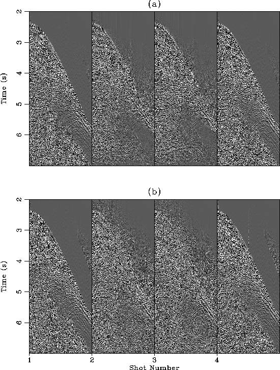
Finally, the interpolated CMP gathers are resorted into shot gathers.
Figure ![[*]](http://sepwww.stanford.edu/latex2html/cross_ref_motif.gif) displays four shot gathers after
interpolation. Shots one and four are original shots from the survey
while shots two and three are new. Note that the near offset traces
have been interpolated for all the shots (known and interpolated).
Similar to what we observed in the CMP domain, the Cauchy
regularization helped to preserve the steep dips better in Figure
displays four shot gathers after
interpolation. Shots one and four are original shots from the survey
while shots two and three are new. Note that the near offset traces
have been interpolated for all the shots (known and interpolated).
Similar to what we observed in the CMP domain, the Cauchy
regularization helped to preserve the steep dips better in Figure
![[*]](http://sepwww.stanford.edu/latex2html/cross_ref_motif.gif) a. In addition, the noise level is quite high
for the interpolation result without regularization in Figure
a. In addition, the noise level is quite high
for the interpolation result without regularization in Figure ![[*]](http://sepwww.stanford.edu/latex2html/cross_ref_motif.gif) b.
Below 5 s, the interpolation without sparseness constraint gives
better results. However, for the multiple prediction, these events
are of little interest. Overall, despite a fairly coarse acquisition geometry,
the radon-based interpolation yields accurate results for a successful
multiple prediction.
b.
Below 5 s, the interpolation without sparseness constraint gives
better results. However, for the multiple prediction, these events
are of little interest. Overall, despite a fairly coarse acquisition geometry,
the radon-based interpolation yields accurate results for a successful
multiple prediction.
shot-recons
Figure 8 Interpolation results in the shot
domain with (a) and without (b) Cauchy regularization. Shots one and
four are known while shots two and three are new. The near offset
traces have been interpolated for all the shots. No AGC has been
applied to these gathers.


Next: Multiple prediction results
Up: Interpolation
Previous: Theory
Stanford Exploration Project
5/5/2005
![[*]](http://sepwww.stanford.edu/latex2html/cross_ref_motif.gif) shows the acquisition
geometry for one particular sail line. The first streamer (shown as 1)
is extracted and used for this field data example.
The ship is moving from right to left. Surface currents
generate strong cable feathering around 642 km in the inline
direction. The receiver positions are displayed for nine shots
only every eight kilometers in Figure
shows the acquisition
geometry for one particular sail line. The first streamer (shown as 1)
is extracted and used for this field data example.
The ship is moving from right to left. Surface currents
generate strong cable feathering around 642 km in the inline
direction. The receiver positions are displayed for nine shots
only every eight kilometers in Figure ![[*]](http://sepwww.stanford.edu/latex2html/cross_ref_motif.gif) .
.
