Testing the Spitz approximation

Now I assume that only a model of the multiples is known. The Spitz approximation in equation () shows how the PEFs for the signal can be estimated. The primaries are recovered with 2-D and 3-D filters. Figure displays two constant offset sections after multiple attenuation with 2-D and 3-D PEFs. 3-D PEFs give by far the best results and attenuate multiples very well.

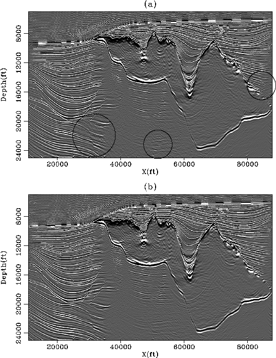
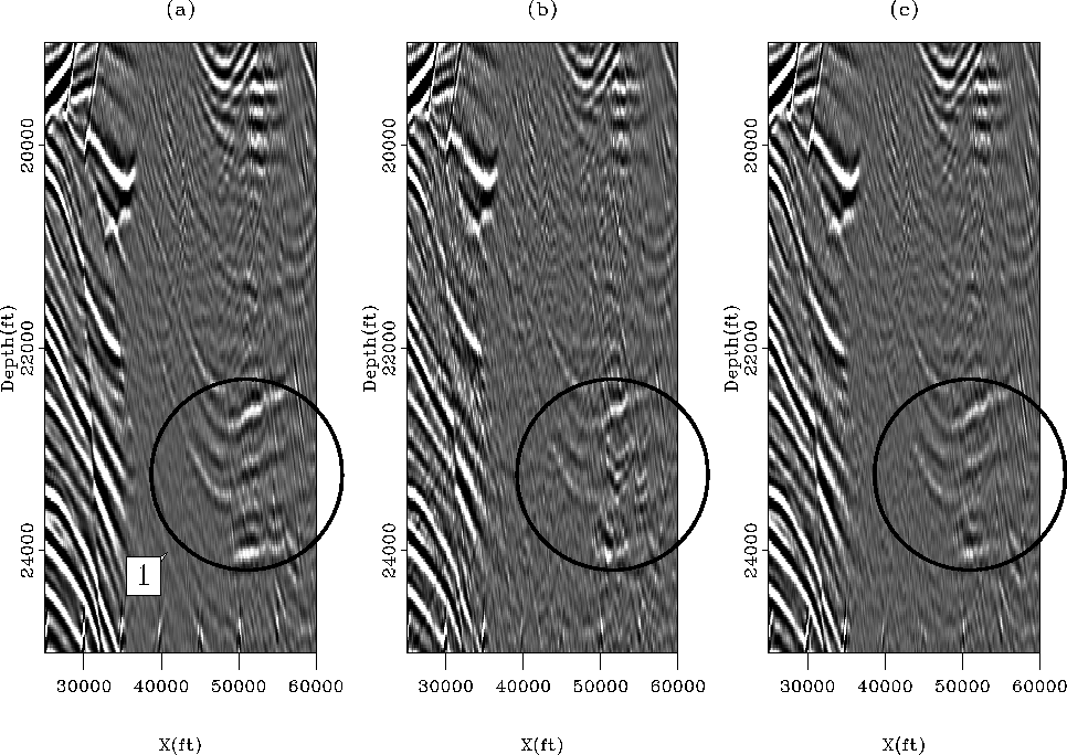
After migration, we see again in Figure that the 3-D PEFs attenuate the multiples more effectively. The circles in Figure surround areas where the 3-D filters are the most effective. A close-up in Figure demonstrates in more detail (e.g., within the circles) how the two results with 2-D or 3-D filters differ below the salt. Events are more continuous and preserved better with 3-D filters. Comparing with the true reflectors in Figure a, important primaries (shown at '1' in Figure a) are attenuated with both 2-D and 3-D filters.

These important observations could not have been made before migration in the prestack domain because the primaries are much weaker than the surface-related multiples below the salt. This illustrates that for complex geology, the quality of a multiple removal technique should be assessed in the image space as often as possible. The fact that some primaries are attenuated in Figure should motivate us in devising improved strategies for building more accurate noise and signal models.

The fact that 3-D PEFs attenuate the multiples better than 2-D PEFs is not surprising. With higher dimensions, primaries and multiples are less likely to be correlated. Therefore, the noise and signal PEFs are less prone to annihilate similar data components. This is particularly important with the Spitz approximation which implicitly assumes that primaries and multiples are uncorrelated.

The next section compares the pattern-based approach with adaptive subtraction on a synthetic dataset provided by BP.

 

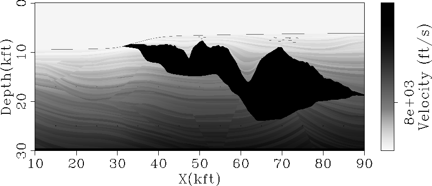
stratigraphy
Figure 2 Stratigraphic interval velocity model of the Sigsbee2B dataset.

 

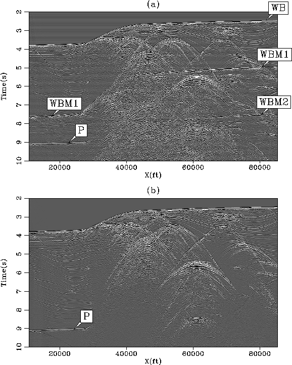
datasignal
Figure 3 Two constant offset sections (h=1125 ft) of the Sigsbee2B dataset with (a) and without (b) free surface condition. The multiples are very strong below 5 s. The weak horizontal striping in (a) comes from a source effect only present with the free surface condition modeling. Arrow WB shows the water-bottom reflection, WBM1 the first order surface-related multiple for the water-bottom, WBM2 the second order surface-related multiple for the water-bottom, and P a strong primary.

 

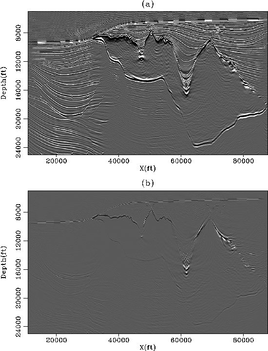
datasignal-mig
Figure 4 Migrated images at zero-offset for the data with (a) and without (b) free surface condition. Comparing with Figure , the multiples appear much weaker below the salt after migration. However, some reflectors near 22 kft are hidden in (a). Arrow WBM1 shows the first order water-bottom multiple after migration. Arrow N shows some noise associated with the migration of multiples beneath the salt body.

 

signal-true
Figure 5 Two constant offset panels at h=1125 ft. for (a) the estimated primaries and (b) the difference with the true primaries. The true primaries and multiples are used to estimate the PEFs. Arrow P shows a primary that could be mistaken for a multiple.

 

signal-true-mig
Figure 6 (a) Migration result after multiple attenuation when the true primaries and multiples are used to estimate the PEFs. (b) Difference between (a) and Figure b. The estimated primaries are almost exact.

 

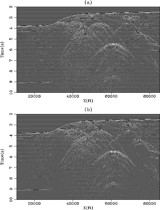
signal-2D-3D-PEF
Figure 7 Two constant offset sections (h=1125 ft) after multiple attenuation with the Spitz approximation using (a) 2-D and (b) 3-D filters.

 

signal-2D-3D-PEF-mig
Figure 8 Two migration results of the estimated primaries with (a) 2-D and (b) 3-D filters. The circles show areas where multiples are better attenuated with 3-D filters than with 2-D filters.

 

signal-2D-3D-PEF-small-mig
Figure 9 Close-up of Figure showing two migrated images when (b) 2-D and (c) 3-D filters are used. The true primaries are shown in (a). Arrow '1' points to primaries that are attenuated with the pattern-based approach. The circles show an area where the 3-D filters are the most effective at removing the multiples.