


Next: Multiple attenuation
Up: Multiple attenuation: Theory and
Previous: Filter estimation
For multiple attenuation, non-stationary PEFs  and
and
 for the multiples and the primaries, respectively, are
needed. Therefore, models for the noise and the signal are necessary.
For surface-related multiples, the multiple model may be
provided by Surface-Related Multiple Prediction (SRMP)
van Dedem (2002); Verschuur et al. (1992), which yields kinematically correct
prestack model of the multiples, especially with 2-D data (see Appendix
for the multiples and the primaries, respectively, are
needed. Therefore, models for the noise and the signal are necessary.
For surface-related multiples, the multiple model may be
provided by Surface-Related Multiple Prediction (SRMP)
van Dedem (2002); Verschuur et al. (1992), which yields kinematically correct
prestack model of the multiples, especially with 2-D data (see Appendix
![[*]](http://sepwww.stanford.edu/latex2html/cross_ref_motif.gif) for details). In 3-D, with marine
acquisition geometry, the crossline offsets need to be heavily
interpolated first. The interpolation results have then a direct impact
on the prediction, as illustrated in Chapter .
for details). In 3-D, with marine
acquisition geometry, the crossline offsets need to be heavily
interpolated first. The interpolation results have then a direct impact
on the prediction, as illustrated in Chapter .
Amplitude-wise, an accurate surface-related multiple model can be derived
if (1) the source wavelet is known, (2) the surface
source and receiver coverage is large and dense enough, and (3) all the terms of the
series that model different orders of multiples
are incorporated Verschuur et al. (1992). Often in practice, a single
convolution of the input data (i.e., one term of the series)
is usually performed, giving a multiple model with erroneous
relative amplitudes for high-order multiples (see Appendix
, equation ()).
Dragoset and Jericevic (1998) detail the possible flaws introduced in
the prediction due to acquisition parameters.
Because PEFs estimate patterns, incorrect
relative amplitudes and kinematic errors can affect multiple
suppression. However, as we shall see later, 3-D filters
seem to cope better with noise modeling inadequacies.
Signal PEFs are more difficult to estimate since the primaries
are usually unknown. As a possible solution to this problem, Spitz (1999) estimates
a signal PEF by deconvolving a data PEF  , estimated
from the data, by a noise PEF . With this process, Spitz assumes that
, estimated
from the data, by a noise PEF . With this process, Spitz assumes that
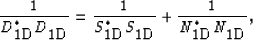
|  |
(51) |
I call equation () the Spitz approximation.
Note that , , and are matrices
for the combinations with the non-stationary PEFs
Margrave (1998). These matrices are very sparse
and are never formed in practice Claerbout and Fomel (2002).
Equation () can be retrieved by considering a simple 1-D example
using the Z-transform notations Claerbout (1976) for a data PEF  ,a signal PEF
  , and a noise PEF
  . Extension to more
dimensions is straightforward using the helical boundary conditions
Claerbout and Fomel (2002). Because PEFs have the inverse
spectrum of the data from which they have been estimated Burg (1975),
we have (omitting Z for clarity purposes)
. Extension to more
dimensions is straightforward using the helical boundary conditions
Claerbout and Fomel (2002). Because PEFs have the inverse
spectrum of the data from which they have been estimated Burg (1975),
we have (omitting Z for clarity purposes)
|  |
(52) |
where (*) is the complex conjugate. Equation
() simply states
that the spectrum of the data is equal to the spectrum of the noise
plus the spectrum of the signal. Equation () can be written as follows:
|  |
(53) |
Now, because PEFs are important where they are small (i.e., where they
attenuate seismic events), the denominator
can be neglected:
|  |
(54) |
which leads to the Spitz approximation in equation ().
The PEFs and can be easily estimated because the
data vector and a noise model are often available. However, estimating
the signal PEFs requires a potentially unstable non-stationary
deconvolution  Rickett (2001) in equation
().
To avoid the deconvolution step, the noise PEFs are convolved with the data:
Rickett (2001) in equation
().
To avoid the deconvolution step, the noise PEFs are convolved with the data:
|  |
(55) |
where  is the result of the convolution. Estimating the PEFs
 for gives by definition of the PEFs Claerbout and Fomel (2002):
|  |
(56) |
Then, from the Spitz approximation in equation
(), we have
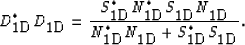
|  |
(57) |
and  . Therefore, by convolving the data with the noise
PEFs, signal PEFs consistent with the Spitz approximation can be
computed. Again, an important assumption is that signal and noise
are uncorrelated. The PEFs for the primaries () and the multiples
() are estimated directly from the data and the model
of the multiples. These filters approximate the multidimensional
spectra of the noise and signal.
. Therefore, by convolving the data with the noise
PEFs, signal PEFs consistent with the Spitz approximation can be
computed. Again, an important assumption is that signal and noise
are uncorrelated. The PEFs for the primaries () and the multiples
() are estimated directly from the data and the model
of the multiples. These filters approximate the multidimensional
spectra of the noise and signal.
Next: Multiple attenuation
Up: Multiple attenuation: Theory and
Previous: Filter estimation
Stanford Exploration Project
5/5/2005