| |
(26) |
![[*]](http://sepwww.stanford.edu/latex2html/cross_ref_motif.gif) .
One possible strategy, however, consists in computing the ratio of the norm (in a
.
One possible strategy, however, consists in computing the ratio of the norm (in a
| (27) |
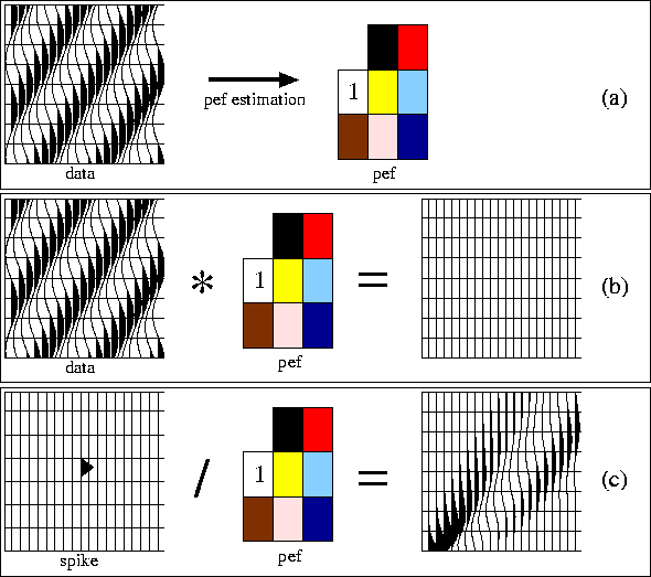
PEFs can play this role as well because they have the
inverse spectrum of the data from which they were estimated. As an
illustration, Figure ![[*]](http://sepwww.stanford.edu/latex2html/cross_ref_motif.gif) a displays a simple monochromatic
plane wave with a given dip. If a multidimensional PEF is estimated
from this dataset, then the PEF will kill this plane wave
(Figure
a displays a simple monochromatic
plane wave with a given dip. If a multidimensional PEF is estimated
from this dataset, then the PEF will kill this plane wave
(Figure ![[*]](http://sepwww.stanford.edu/latex2html/cross_ref_motif.gif) b). Now, looking at the inverse
impulse response of this filter (i.e., deconvolution) in
Figure
b). Now, looking at the inverse
impulse response of this filter (i.e., deconvolution) in
Figure ![[*]](http://sepwww.stanford.edu/latex2html/cross_ref_motif.gif) c, notice that an event with similar
frequency content and dip than in Figure
c, notice that an event with similar
frequency content and dip than in Figure ![[*]](http://sepwww.stanford.edu/latex2html/cross_ref_motif.gif) a is
recovered. Thus, PEFs can serve as either filters when convolved with
the residual (filtering approach) or modeling operators when used with
deconvolution.
a is
recovered. Thus, PEFs can serve as either filters when convolved with
the residual (filtering approach) or modeling operators when used with
deconvolution.
PEFs are minimum-phase filters Claerbout (1976); Robinson and Treitel (2000), which makes their inverse (with deconvolution) stable. In the stationary case where one filter is needed, inverse PEFs can play the role of modeling operators, and strategies similar to the one used for the filtering approach can be employed to estimate them. In the non-stationary case, however, the non-stationary deconvolution of minimum-phase filters is not guaranteed to be stable Rickett (2001). This defect prevents us from reliably using inverse non-stationary PEFs as modeling operators.
|
fbpef
Figure 1 Some basic properties of the prediction-error filters (PEF). (a) A PEF is estimated from a dataset. (b) The estimated PEF is convolved with the input data leading to a white residual. (c) A spike is deconvolved with the estimated PEF leading to a pattern close to the input data in (a). |  |