Application to the dip estimation problem

The goal of dip estimation is to find a local stepout, $\sigma$, that destroys the local plane wave such that,

$$0 \approx \frac{\partial u}{\partial h} + \sigma \frac{\partial u}{\partial \tau},$$ (9)

where u is the wavefield at time $\tau$ and offset h. For all gathers, we evaluate the slope $\sigma$ with a method based on high-order plane-wave destructor filters Fomel (2002). With the Z transform notation, Fomel (2002) shows that there is a 2-D filter

 

C_n(Z_t,Z_h)=B_n(Z_t^-1)-Z_hB_n(Z_t), (10)

with

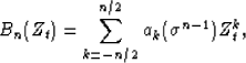
$$B_n(Z_t)=\sum_{k=-n/2}^{n/2}a_k(\sigma^{n-1})Z_t^{k},$$ (11)

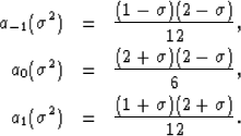
that annihilates the local plane wave. The number of coefficients for the filter B_n is n. The filter coefficients $a_k(\sigma^{n-1})$ are functions of $\sigma^{n-1}$ as detailed in equations (9) and (10) of Fomel (2002). For instance, if n=3, we have

$$\begin{eqnarray} a_{-1}(\sigma^2)&=&\frac{(1-\sigma)(2-\sigma)}{12},\nonumber \\... ...,\\ a_{1} (\sigma^2)&=&\frac{(1+\sigma)(2+\sigma)}{12}.\nonumber \end{eqnarray}$$ (12)

In equation (11), $\sigma$ is unknown and is estimated with a non-linear solver.
 

• Inversion