REFERENCES

Broyden, C. G., 1969, A new double-rank minimization algorithm: AMS Notices, 16, 670.

Conn, A. R., Gould, N. I. M., and Toint, P. L., 1992, LANCELOT: A Fortran package for large-scale nonlinear optimization (Release A): Springer Series in Computational Mathematics 17.

Fletcher, R., 1970, A new approach to variable metric methods: Comput. J., 13, 317-322.

Fomel, S., 2002, Applications of plane-wave destruction filters: Geophysics, 67, no. 06, 1946-1960.

Goldfarb, D., 1970, A family of variable metric methods derived by variational means: Math. Comp., 24, 23-26.

Guitton, A., and Symes, W., 2003, Robust inversion of seismic data using the Huber norm: Geophysics, 68, no. 4, 1310-1319.

Kelley, C. T., 1999, Iterative methods for optimization: SIAM in applied mathematics.

Liu, D. C., and Nocedal, J., 1989, On the limited memory BFGS method for large scale optimization: Mathematical Programming, 45, 503-528.

Lomask, J., 2003, Flattening 3D seismic cubes without picking: Soc. of Expl. Geophys., 73rd Ann. Internat. Mtg., 1402-1405.

Nocedal, J., 1980, Updating quasi-Newton matrices with limited storage: Mathematics of Computation, 95, 339-353.

Sava, P., and Guitton, A., 2003, Multiple attenuation in the image space: Soc. of Expl. Geophys., 73rd Ann. Internat. Mtg., 1933-1936.

Shanno, D. F., 1970, Conditioning of quasi-Newton methods for function minimization: Math. Comp., 24, 647-657.

Zhu, H., Byrd, R. H., and Nocedal, J., 1997, Algorithm 778: L-BFGS-B, FORTRAN routines for large scale bound constrained optimization: ACM Transactions on Mathematical Software, 23, 550-560.

 

fabricposneg
Figure 1 (a) Input data. (b) Estimated dips with L-BFGS-B without bound constraints. (c) Estimated positive dips only. (d) Estimated negative dips only.

 

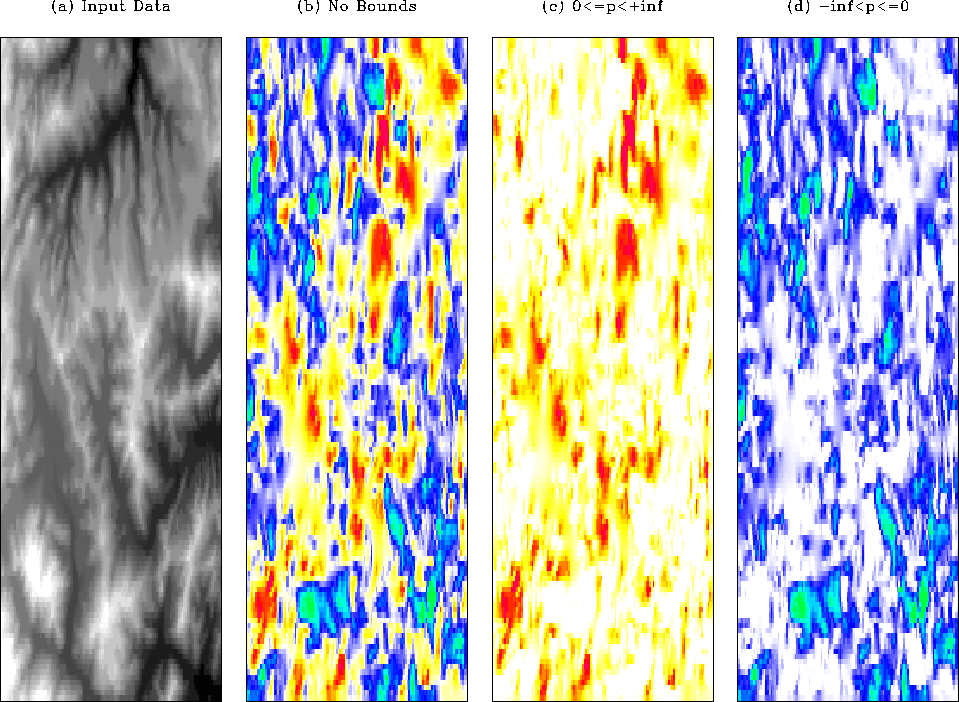
sfbayposneg
Figure 2 (a) Input data. This topographic map comes from the bay area. (b) Estimated dips with L-BFGS-B without bound constraints. (c) Estimated positive dips only. (d) Estimated negative dips only.

 

aliasposneg
Figure 3 (a) Input data. (b) Estimated dips with L-BFGS-B without bound constraints. (c) Estimated positive dips only. (d) Estimated negative dips only. Positive and negative dips are found beyond aliasing.

 

dipposneg
Figure 4 (a) Input data. The lines cross at a location where the dips should be positive. (b) Estimated dips with L-BFGS-B without bound constraints. Negative dips are actually found at the crossing of the lines. (c) Estimated positive dips only. The bound constrained optimization is capable of identifying the true positive dips. (d) Estimated negative dips only.

 

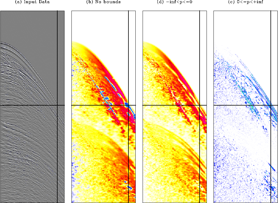
gmdip
Figure 5 (a) Input data. (b) Estimated dips with L-BFGS-B without bound constraints. At the cross, negative dips are given although only positive dips should be found. (c) Estimated positive dips only. Positive dips are recovered everywhere. (d) Estimated negative dips only.

 

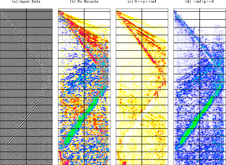
idaposneg
Figure 6 (a) Input data. The cross shows a location where two events overlap. (b) Estimated dips with L-BFGS-B without bound constraints. (c) Estimated positive dips only. At the cross, no positive dips are estimated because the overlapping event that goes in the other direction is too strong. (d) Estimated negative dips only.

 

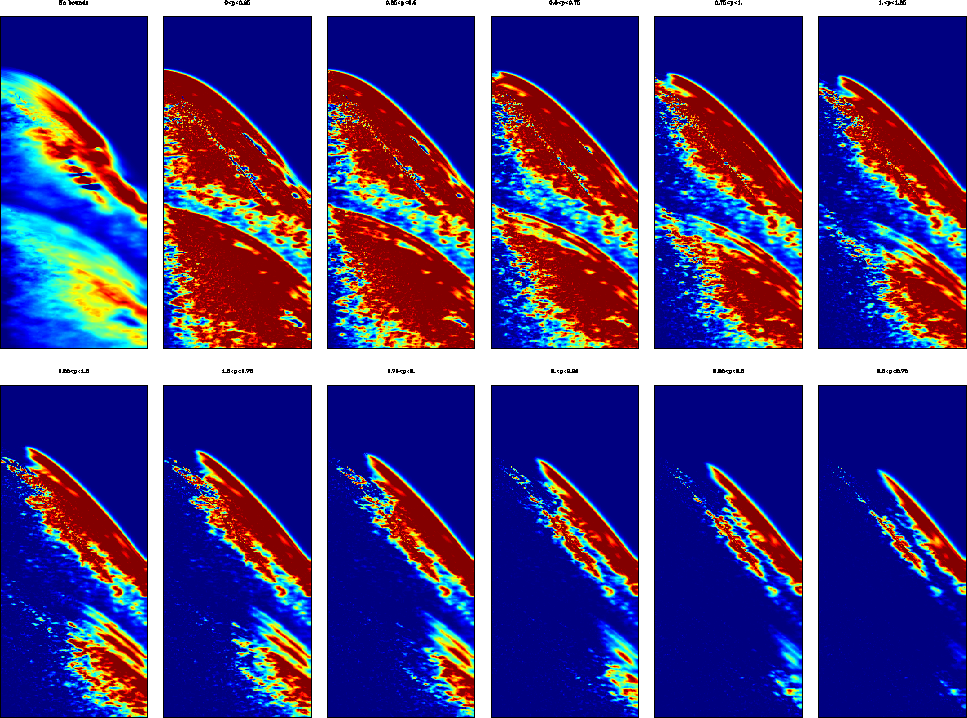
gmdecomp
Figure 7 The fist panel on the top left corner shows the dips without the bounds. Then, from left to right, top to bottom, the range of dip increases by 0.25 between each panel, starting at $0 \leq \sigma \leq 0.25$ and finishing at $2.5 \leq \sigma \leq 2.75$. The lower and upper clip values are equal to the bounds for each panel.