LSJIMP versus Radon Demultiple

Radon demultiple remains the default multiple suppression technique in many situations, particularly in 3-D, where acquisition sparsity may inhibit other techniques. On CMP gathers, primaries and multiples normally have different apparent velocities, and a Radon transform which sums across offset using various curvature parameters will focus the two types of events in different parts of the transform panel. The most natural curvature parameter for CMP data is the velocity of the hyperbola defined by the NMO equation Foster and Mosher (1992). While the Hyperbolic Radon transform is a linear mapping, it is not time-invariant, and thus cannot be implemented efficiently as a Fourier domain operator. However, a multiple's residual moveout after NMO is approximately parabolic (quadratic) with offset, so a time-invariant Parabolic Radon transform is much faster, though not as accurate Hampson (1986); Kabir and Marfurt (1999).

To remove multiples, the multiple energy in the transform panel is muted, and the inverse Radon transform applied to produce multiple-free CMP data. If we define $\bf d$ as a raw CMP gather, $\bf H$ as the linear mapping between Radon transform space and data space, $\bf M$ as a mute operator that zeroes multiple energy in Radon transform space, and $\bold d_r$ as the estimated primaries, then we can express the Radon demultiple process in equation form:  

$$\bold d_r = \bold H \bold M^T \bold H^T \bold d.$$ (6)

Operator $\bf H$ is non-unitary ($\bold H^T \bold H \neq \bold I$), so the amplitude of the estimated primaries will not match the recorded primaries. By casting Radon demultiple as a least-squares optimization problem, the Radon transform panel can be scaled such that $\bold d_r$ and $\bf d$ are directly comparable. We first optimize a Radon transform panel, $\bf p$, to minimize the data misfit:  

$$\mbox{ \raisebox{-1.0ex}{ $\stackrel{\textstyle \mbox{\LARGE... ... \bold p} $} } Q(\bold p) \; = \; \Vert {\bf Hp - d } \Vert^2,$$ (7)

and then apply the mute operator and adjoint of $\bf H$ to produce the estimated primaries:  

$$\bold d_r = \bold H \bold M^T \bold p.$$ (8)

The finite frequency content of the data, limited extent of the array, and the intrinsic unresolvability of velocity information at zero offset all contribute to the non-uniqueness of the least-squares Radon demultiple problem. At far offsets, events with many zero-offset traveltimes and different velocities are fit equally well by a single curvature parameter. Low-frequency data makes moveout discrimination between multiples and primaries more difficult. At near offsets, all the events are fit equally well by all curvature parameters. All these pitfalls lead to reduced resolution of events in the Radon domain. So-called ``high resolution'' least-squares Radon transform implementations partially overcome these problems by imposing sparsity constraints in either the hyperbolic or parabolic Radon domain Sacchi and Ulrych (1995); Thorson and Claerbout (1985).

I implemented and tested least-squares Hyperbolic Radon demultiple (LSHRTD) on the CGG 3-D data subset. I performed 10 conjugate gradient iterations to produce an optimal $\bf p$, then applied a mute function which is zero for velocities less than 85% and greater than 115% of the known stacking velocity. The mute tapers linearly from 0.0 to 1.0 at 90% and 110% of the known stacking velocity, respectively. The computational cost of LSHRTD is very similar to the cost of applying LSJIMP.

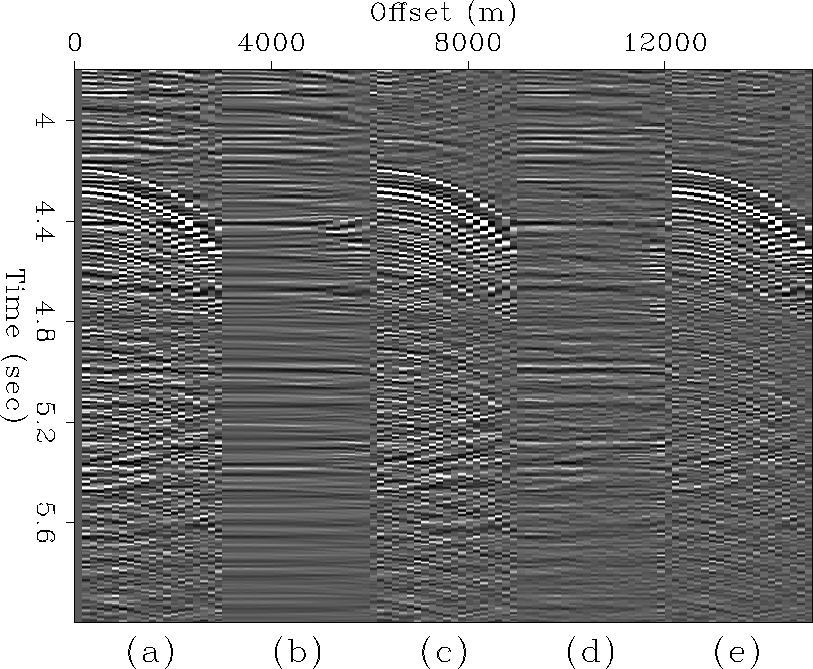
Figure 10 compares the results of applying LSJIMP and LSHRTD on a single CMP gather from the CGG 3-D data (CMPx=100, CMPy=4). The LSHRTD results are quite good, as we expect, given the high velocity gradient and relatively simple moveout seen in this region of the data. Note some ``smearing'' of primaries in the LSHRTD result, as well as a generally higher level of energy removed from the data. Both effects would likely be lessened by a more conservative, tapered mute. LSJIMP is a more ``surgical'' separation technique, although the model regularization operators also exploit moveout differences to separate multiples and primaries.

 

comp.radon.gc3d.100
Figure 10 LSJIMP versus least-squares Hyperbolic Radon demultiple (LSHRTD) on one CMP gather of the CGG 3-D dataset. Panel (a): Raw data. Panel (b): LSHRTD estimated primaries. Panel (c): LSHRTD estimated multiples. Panel (d): LSJIMP estimated primaries. Panel (e): LSJIMP estimated multiples.

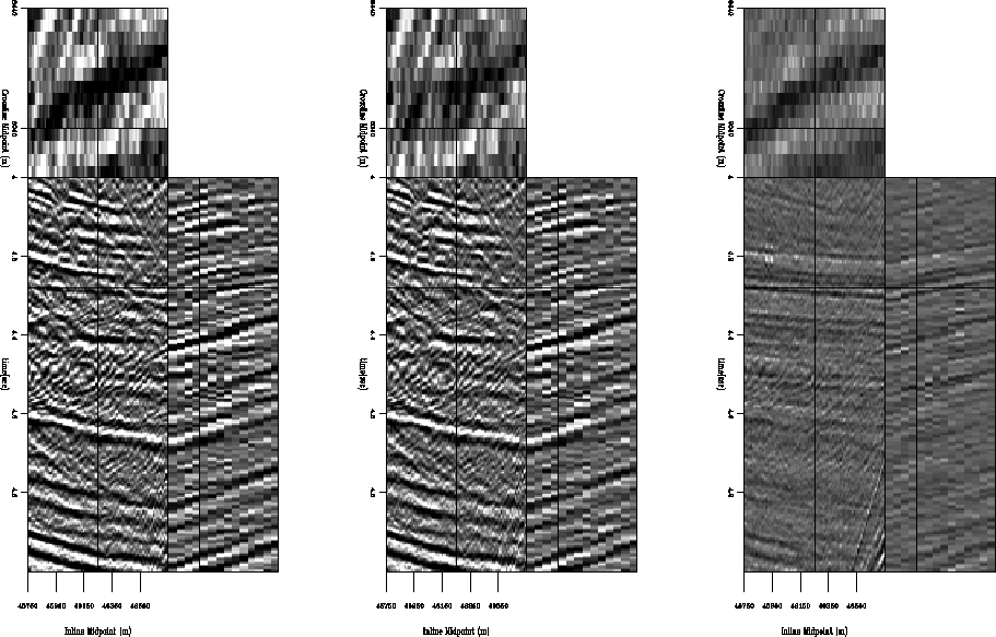
Figure 11, a stack of the LSHRTD estimated primaries, can be compared directly with the LSJIMP result, Figure 7. Like before, the multiples predominantly stack out, since the moveout separation is so significant. Still, a noticeable amount of multiple energy has been removed by LSHRTD, perhaps more than by LSJIMP. However, we immediately see some removed primary energy: for example, the strong primary near the bottom of the section.

 

stackcomp3d.radon.zoom.gc3d
Figure 11 NMO/Stack comparison before and after LSHRTD. Compare directly with Figure 7. Left: Raw data. Center: LSHRTD estimated primaries. Right: difference.