Results

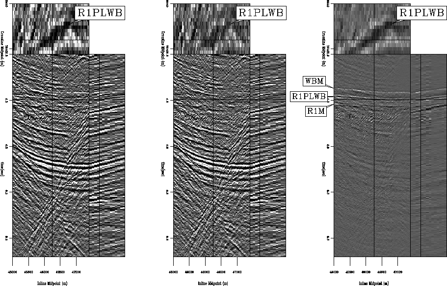
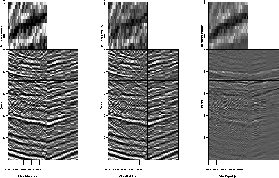
Figure 6 shows stacked sections from the multiple-infested zone of the CGG subset before and after application of LSJIMP. Figure 7 is in the same format, but shows a zoom of the multiple-infested region. CMP stacking strongly suppresses the multiples, but from the difference panel, notice that LSJIMP has nonetheless subtracted most of the remaining surface-related multiple energy, and has preserved the stronger primaries to a great extent. The timeslice on the 3-D cube transects the seabed pegleg from reflector R1; it shows up prominently on the raw data stack, as well as on the difference panel, but has been largely suppressed from the LSJIMP estimated primaries stack.

 

stackcomp3d.gc3d
Figure 6 Stacked subset (192 midpoints inline, 14 midpoints crossline) of CGG 3-D data before and after LSJIMP. All panels windowed in time from 3.8 to 6.0 seconds and gained with t². Left: Raw data stack. Center: Stack of estimated primary image, $\bold m_0$. Right: Stack of the subtracted multiples. Naming convention for pure first-order multiples: (reflector)M, e.g., R1M. Naming convention for first-order pegleg multiples: (target)PL(multiple generator), e.g., R1PLWB.

 

stackcomp3d.zoom.gc3d
Figure 7 Zoom of stacked subset of CGG 3-D data before and after LSJIMP. All panels windowed in time from 4.0 to 5.0 seconds. Left: Raw data stack. Center: Stack of estimated primary image, $\bold m_0$. Right: Stack of the subtracted multiples.

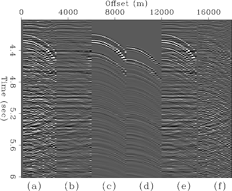
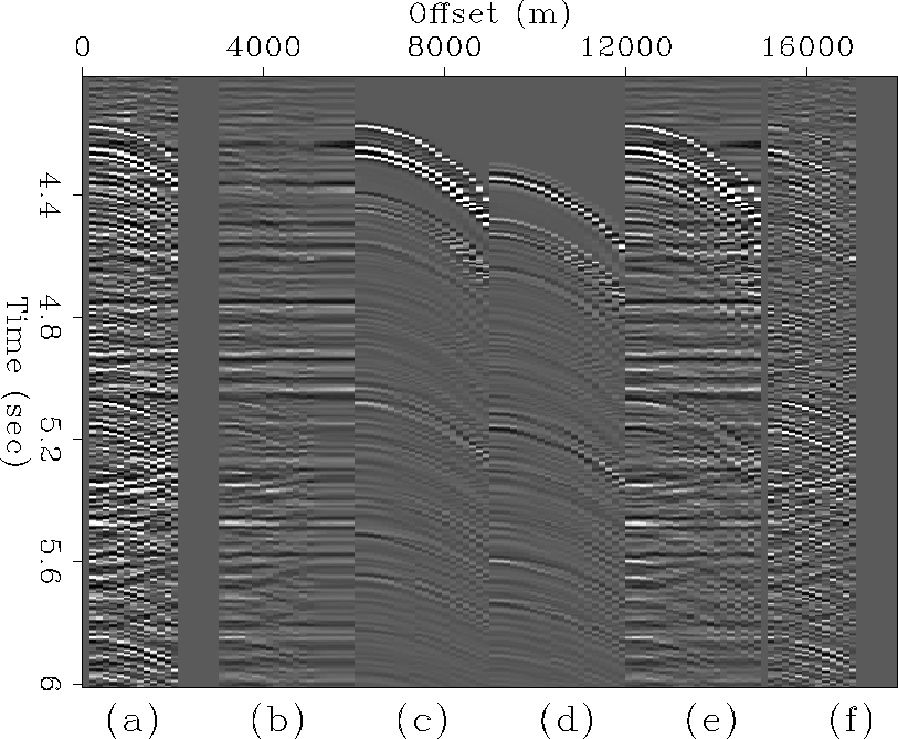
Figures 8 and 9 illustrate LSJIMP's performance on two individual CMP gathers extracted from different portions of the CGG 3-D data. It is in this domain where the strength of the LSJIMP method shines most. The raw data panels show strong surface-related multiples with an onset of around 4.3 seconds, and also fairly strong primary events under the curtain of multiples. The LSJIMP estimated primaries in panel (b) are effectively free of multiples, and moreover, since the data residual panel (f) barely contains any noticeable flat primary energy, we have preserved the primary events. Also notice that the data residual contains little structured energy. This implies that the LSJIMP forward model accurately models the primaries and important multiples in the data. Unfortunately, much of this ``unstructured'' energy likely belongs to fairly weak pegleg multiples that simply appear incoherent with the data's poor inline resolution. On Figure 9, notice that cable feathering has caused missing traces at far offsets. LSJIMP has used the data's multiplicity and model constraints to reasonably extrapolate the missing traces.

 

compwind.lsrow.gc3d.100.4
Figure 8 LSJIMP results on individual midpoint location (CMPx=100,CMPy=4). All panels decimated in offset by a factor of 6 and NMO'ed with stacking velocity, for display purposes. Panel (a): Raw data. Panel (b): LSJIMP estimated primaries. Panels (c) and (d): Estimated seabed and R1 pegleg multiples. Panel (e): Modeled data (sum of panels (b), (c), and (d)). Panel (f): Data residual (difference of panels (a) and (e)), with residual weight applied.

 

compwind.lsrow.gc3d.100.12
Figure 9 LSJIMP results on individual midpoint location (CMPx=100,CMPy=12). All panels decimated in offset by a factor of 6 and NMO'ed with stacking velocity, for display purposes. Panel (a): Raw data. Panel (b): LSJIMP estimated primaries. Panels (c) and (d): Estimated seabed and R1 pegleg multiples. Panel (e): Modeled data (sum of panels (b), (c), and (d)). Panel (f): Data residual (difference of panels (a) and (e)), with residual weight applied.

 

• LSJIMP versus Radon Demultiple
• AVO Analysis Before and After LSJIMP