Next: Discussion-Conclusion
Up: Guitton et al.: Velocity
Previous: Tomography
Figure 1 displays a near-offset section of a
2D dataset. The geology is relatively simple with mostly flat layers and
few normal faults. A first 1D interval slowness model is estimated by
assuming a  function that leads to
 in
in  space.
With this dataset v0=1.6 km/s and
space.
With this dataset v0=1.6 km/s and  . We then transform
the velocity into an interval slowness function shown Figure 2.
near-offset
. We then transform
the velocity into an interval slowness function shown Figure 2.
near-offset
Figure 1 Near-offset section of the 2D field
dataset from the Gulf of Mexico. Some normal faults are visible.

s0
Figure 2 Initial slowness function.
|
| 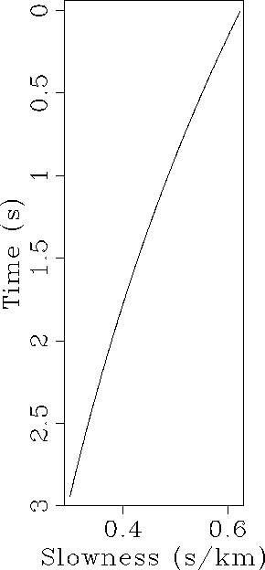 |
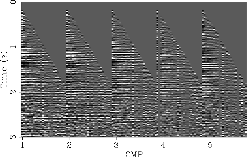
Figure 3 shows every twenty-fifth CMP gathers after NMO
correction. Note that these gathers are not perfectly flat and that
the noise level is quite high, especially in the
deepest part of the section. In addition, there are both missing
and bad traces at different offsets. We expect that the estimation
of stepouts is robust enough to the noise level present in the gathers to
give reasonable dips.
pano.nmo
Figure 3 Five CMP gathers every 1.6 km after NMO correction with
the RMS velocity derived from the interval slowness in Figure
2. Some residual curvature is apparent throughout the section.
Local stepouts and time shifts are estimated from the CMP gathers.
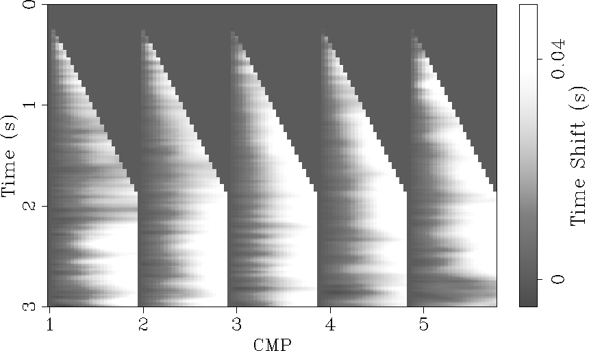
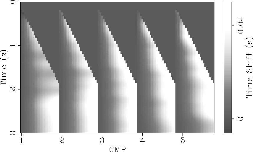
Figure 4 displays the estimated time
shifts for the five selected CMP gathers. It is interesting to notice
that the time shifts increase with offset. The time shifts are also
relatively smooth in the  direction thanks to the dip
regularization in equation (3). The smoothing in both offset
and midpoint directions during the stepouts estimation
allows us to have time shifts where traces were
originally missing (e.g., gathers four and five in Figure
3).
The fact that the estimated time shifts change with midpoint
for a fixed time and offset prove that lateral velocity variations
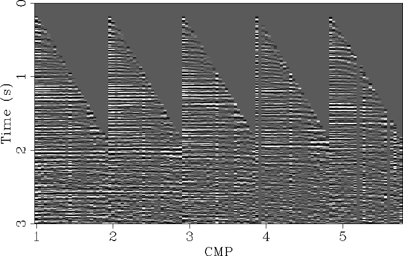
exist. These time shifts can be checked by applying a
moveout correction to the input gathers in Figure 3 according to the
shift values in Figure 4. Figure
5 shows the same gathers after
moveout correction. These gathers are now flat and demonstrate that
the estimated time shifts after integration of the local stepouts are correct.
direction thanks to the dip
regularization in equation (3). The smoothing in both offset
and midpoint directions during the stepouts estimation
allows us to have time shifts where traces were
originally missing (e.g., gathers four and five in Figure
3).
The fact that the estimated time shifts change with midpoint
for a fixed time and offset prove that lateral velocity variations
exist. These time shifts can be checked by applying a
moveout correction to the input gathers in Figure 3 according to the
shift values in Figure 4. Figure
5 shows the same gathers after
moveout correction. These gathers are now flat and demonstrate that
the estimated time shifts after integration of the local stepouts are correct.
time.pano.realshift
Figure 4 Estimated time shifts
for five CMP gathers. The maximum time shift is around 0.05
s. Note that the first trace is set to zero.
pano.data.flat
Figure 5 Flattened CMP gathers
after applying the time shifts in Figure
4. Comparing with Figure
3, most of the events are now flat.
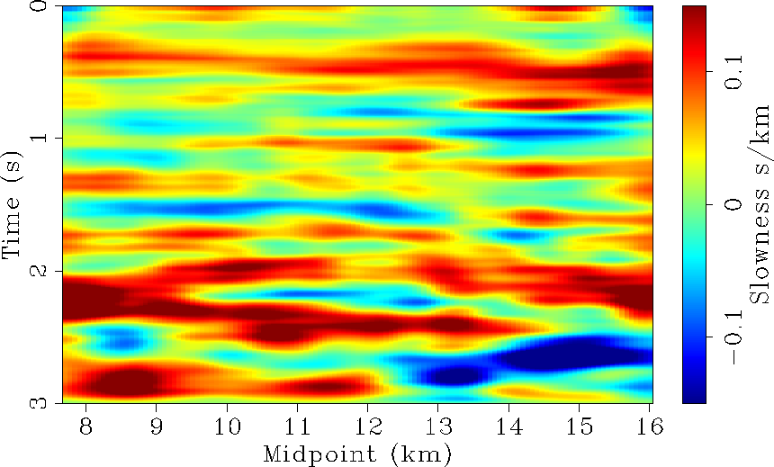
The velocity perturbations are then estimated from the time shifts
with the tomography. Figure 6
shows estimated slowness perturbations and Figure
7 displays the updated slowness field.
We used 40 iterations and set  in equation
(15) to obtain this result.
Lateral velocity variations are visible throughout.
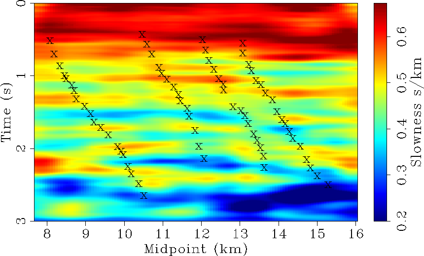
In Figure 8, four fault locations
interpreted from the seismic are superimposed
(Figure 15). These faults locations seem to be
aligned with velocity variations in Figure
7. In particular,
it is pleasing to see the change of velocities across the different
faults.
in equation
(15) to obtain this result.
Lateral velocity variations are visible throughout.
In Figure 8, four fault locations
interpreted from the seismic are superimposed
(Figure 15). These faults locations seem to be
aligned with velocity variations in Figure
7. In particular,
it is pleasing to see the change of velocities across the different
faults.
To check whether the method converged,
modeled time shifts are estimated from the slowness perturbations in
Figure 6 by applying the forward operator
in equation (10). The re-modeled time shifts are shown
in Figure 9.
Comparing Figures 4 and
9, it appears that the re-modeled
time shifts are smoother. Yet, applying these time shifts
to the NMO corrected data in Figure 3 yield
flat gathers (Figure 10). The
difference between Figures 4 and
9 is that the
re-modeled time shifts are constrained by the physics of the
tomographic inversion, thus giving well-behaved amplitude variations.
In Figure 4, however, the time
shifts take any value according to estimated dips. The forward
operator of the tomographic inversion can be interpreted as
a velocity-consistent, time shifts estimator.
delta.dslow
Figure 6 Slowness perturbations
estimated from the tomography in the space.
vel.slowupdate
Figure 7 Updated slowness field by
adding Figures 2 and 6.
velinter.slowupdate
Figure 8 Same as Figure
7 with four interpreted faults from
the seismic. Note the changes of velocity across the faults.
time.pano.newshift
Figure 9 Modeled time shifts
from slowness perturbations in Figure
6. Note that the remodeled time shifts
are smoother than the original ones in Figure 4.
pano.new.data.flat
Figure 10 Flattened data with
the remodeled time shifts in Figure
9. The gathers are flat
showing that the slowness perturbations in Figure
6 fit the estimated time shifts in Figure
4 very well.
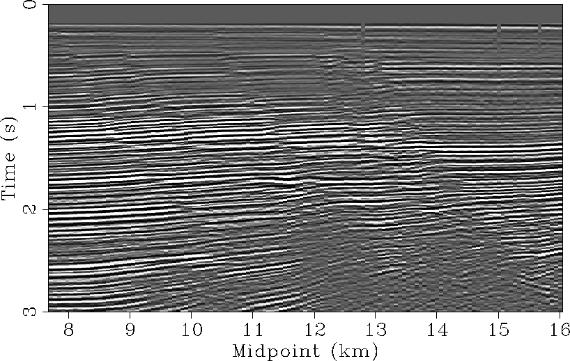
Finally, the flattened gathers in Figure
10 are stacked
(Figure 14).
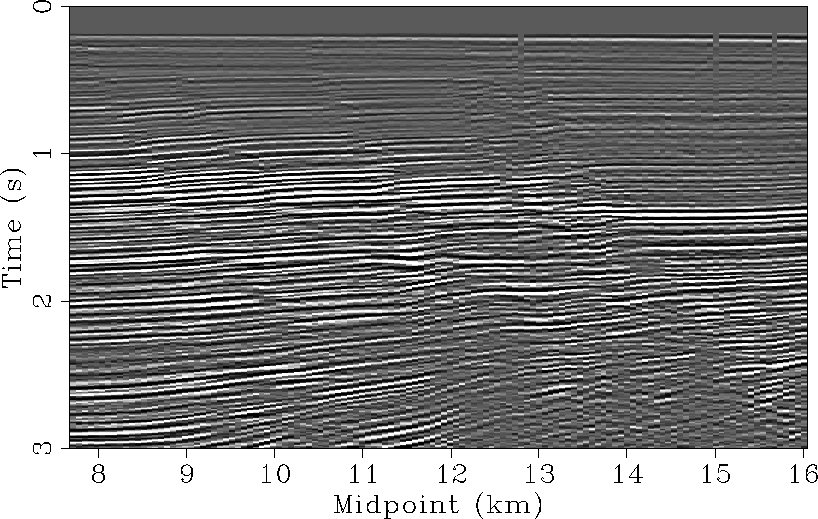
We compare this result with the stacked section of the data with a 1D slowness
model shown in Figure 11. This slowness function flattens the CMP
gathers well for every midpoint position (Figure 12).
We show the stacked section of the input
data with this 1D slowness function in Figure 13.
The reflectors are stronger and better defined in
Figure 14 wherever the signal level is
strong. In the lower part of the section, however, some continuous
events in Figure 13 are attenuated
in Figure 14. This effect is due to the
difficulty to estimate meaningful stepouts when the noise level is too
high. Again, four interpreted faults are shown on the stacked section
in Figure 15.
s1
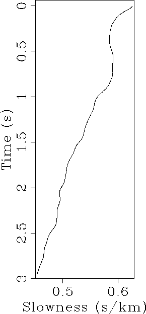
Figure 11 A 1D stacking slowness function.
|
|  |
panos1
Figure 12 CMP gathers after NMO with the slowness function in
Figure 11. The gathers are almost flat.
stack-bestslow
Figure 13 Stacked section of the data with the
our best picked 1D slowness function in Figure 11.
stack.new.data.flat
Figure 14 Stacked section of
the moveout corrected data from the remodeled time shifts in Figure
9.
stackinter.new.data.flat
Figure 15 Stacked section of
the moveout corrected data from the remodeled time shifts in Figure
9 with four picked faults.
Next: Discussion-Conclusion
Up: Guitton et al.: Velocity
Previous: Tomography
Stanford Exploration Project
5/23/2004