Tomography

From the time shifts, we estimate interval velocities in the $\tau$ domain. As pointed out by Alkhalifah (2003) and Clapp (2001), $\tau$ tomography is more robust than depth tomography to reflector position and velocity errors. However, going from depth to vertical travel time introduces new variables. As described by Biondi et al. (1997) and Alkhalifah (2003), the transformation from depth coordinates (x,z) into vertical-traveltime coordinates $(\tilde x,\tau)$ is governed by the relationships:

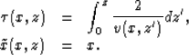$$\begin{array} {rcl} \tau(x,z) &=& \displaystyle \int_0^z \frac{2}{v(x,z')}dz', \\ \tilde x(x,z) &=& x. \end{array}$$ (7)

Therefore, we have the following relationships between the differential quantities (dx,dz) and $(d\tilde x,d\tau)$:

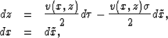$$\begin{array} {rcl} dz &=& \displaystyle \frac{v(x,z)}{2} d... ...v(x,z) \sigma}{2} d\tilde x, \\ dx &=& d\tilde x, \end{array}$$ (8)

where v(x,z) is the focusing velocity proportional to the mapping velocity Clapp (2001) and

$$\sigma = \int_0^z \frac{\partial}{\partial x}\left (\frac{2}{v(x,z')}\right ) dz'.$$ (9)

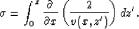
In this paper, it is assumed that $x=\tilde x$ and $\sigma=0$ because the initial slowness field is horizontally invariant.

The data space for this inverse problem is a cube of time-shifts at every time, offset and midpoint location. This differs from most tomographic techniques where a few reflectors are usually selected and picked for the inversion. The number of the model space unknowns (the velocity update) is the product of the number of gathers and the number of time samples. A velocity perturbation is computed for each pixel in the model space. 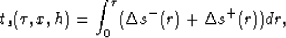For a CMP location x at time $\tau$ and offset h, a total time shift t_s is estimated. The forward problem relating velocity perturbation and time shift is derived from Fermat's principle:  

$$t_s(\tau,x,h)=\int_0^{\tau} (\Delta s^-(r)+ \Delta s^+(r)) dr,$$ (10)

with

$$dr = \frac{d(dt)}{dS},$$ (11)

where $\Delta s^-(r)$ and $\Delta s^+(r)$ are the slowness perturbations along the down- and up-going rays respectively (from x-h/2 to x and x+h/2 to x), S is the focusing slowness, and dt the time increment along the ray Clapp and Biondi (2000). Note that slownesses are actually estimated and not velocities, as it is usually done in tomography. To simplify the problem, we assume that the up- and down-going rays are straight lines in the $(\tau,x)$ space.

Equation (10) is a linear relationship between the time shifts and the slowness perturbations allowing us to write,

$${\bf d} = {\bf Lm},$$ (12)

where ${\bf d}$ are the estimated time shifts, ${\bf L}$ is the tomographic operator in equation (10) and ${\bf m}$ is a field of slowness perturbations. Our goal is to find ${\bf m}$ such that,

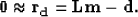$${\bf 0} \approx {\bf r_d} = {\bf Lm-d}.$$ (13)

The addition of a regularization operator to enforce smoothness in the horizontal direction gives:

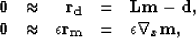$$\begin{array} {ccrcl} {\bf 0} & \approx & {\bf r_d} & = & {... ... \epsilon{\bf r_m} & = & \epsilon \nabla_x{\bf m}, \end{array}$$ (14)

where $\nabla_x$ is the horizontal gradient. Next, ${\bf m}$ is estimated in a least-squares sense by minimizing objective function,  

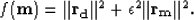$$f({\bf m})=\Vert{\bf r_d}\Vert^2+\epsilon^2\Vert{\bf r_m}\Vert^2.$$ (15)

In practice, ${\bf m}$ is estimated with a conjugate-gradient method and $\epsilon$ is estimated by trial and error. Because tomography is inherently non-linear, more iterations are needed to converge toward a satisfying velocity model. However, the assumptions made in this paper do not allow us to iterate without using more sophisticated imaging operators or ray tracing tools. We now test our method on a 2D Gulf of Mexico dataset.