


Next: Finite-difference solutions to the
Up: Sava and Fomel: Riemannian
Previous: One-way wave-equation in 3-D
We can use equation (12) to construct a numerical solution
to the one-way wave equation in the mixed
 ,
,  domain.
The extrapolation wavenumber described in equation (12)
is, in general, a function which depends on several quantities
domain.
The extrapolation wavenumber described in equation (12)
is, in general, a function which depends on several quantities
| 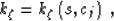 |
(14) |
where  is the space-variable slowness, and
 are
coefficients which are computed numerically from the definition
of the coordinate system, as indicated by
equations (8).
For any given coordinate system,
are
coefficients which are computed numerically from the definition
of the coordinate system, as indicated by
equations (8).
For any given coordinate system,  can be regarded as known.
Next, we write the extrapolation wavenumber  as a
first-order Taylor expansion relative to a reference medium:
as a
first-order Taylor expansion relative to a reference medium:
|  |
(15) |
where and  represent the spatially variable slowness and coordinate
system parameters, and
represent the spatially variable slowness and coordinate
system parameters, and  and
and  are the
constant reference values in every
extrapolation ``slab'' Sava (2000).
are the
constant reference values in every
extrapolation ``slab'' Sava (2000).
As usual, the first part of equation (15),
corresponding to the extrapolation wavenumber in the
reference medium  ,is implemented in the Fourier domain,
while the second part, corresponding to the spatially variable
medium coefficients, is implemented in the space domain.
,is implemented in the Fourier domain,
while the second part, corresponding to the spatially variable
medium coefficients, is implemented in the space domain.
If we make the further simplifying assumptions that
 and
and  ,
we can write
,
we can write
| 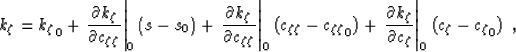 |
(16) |
where
| 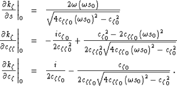 |
|
| |
| (17) |
Equation (16) is motivated by
a wavefront normal propagation approximation.
By ``0'', we denote the reference medium ( .We could also use many reference media, followed by
interpolation, similarly to the technique of
Gazdag and Sguazzero (1984).
.We could also use many reference media, followed by
interpolation, similarly to the technique of
Gazdag and Sguazzero (1984).
For the particular case of Cartesian coordinates
( ),
equation (16) reduces to
),
equation (16) reduces to
|  |
(18) |
which corresponds to the popular Split-Step Fourier (SSF)
extrapolation method Stoffa et al. (1990).
Next: Finite-difference solutions to the
Up: Sava and Fomel: Riemannian
Previous: One-way wave-equation in 3-D
Stanford Exploration Project
10/14/2003