Subtracting the coherent noise in synthetic data

For this first series of tests, I used the synthetic data in Figure 1. The first stage, after which I estimate a PEF from the residual, took 45 iterations. The filter is one-dimensional with 30 coefficients (a=30,1). In the second stage, I use the inverse of the filter as the noise modeling operator shown in equation (4).

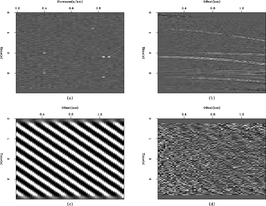
The subtraction results in a reduction of the noise similar to that with the filtering method. Figure 13 shows the result of the inversion. The residual (Figure 13d) is white, the model space is well resolved with all the curvatures present (Figure 13a), and the noise model (Figure 13c) clearly displays the linear coherent noise. The top and bottom of the residual (Figure 13d) were masked to avoid edge effects caused by the helical boundary conditions. Figure 13b shows the reconstructed data. 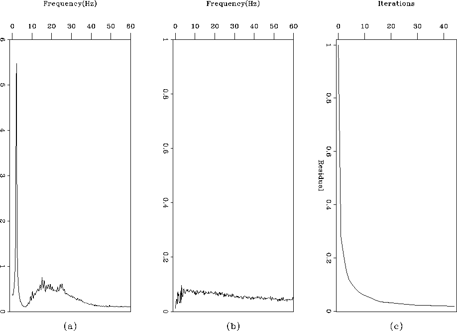This result compares favorably with that in Figure 3b. Finally, Figure 14a compares the amplitude spectrum of the input data (Figure 14a) and of the residual (Figure 14b). Obviously, the residual energy is very small.

 

compsy
Figure 13 Subtracting the coherent noise in synthetic data. (a) An estimated model space. (b) The reconstructed data from the model space. (c) The estimated coherent noise ${\bf A_n^{-1}m_n}$. (d) The residual after inversion. Click Movie to see how the four panels evolve as the iterations continue.

 

compsf
Figure 14 (a) The amplitude spectrum of the input data in Figure 1a. (b) The amplitude spectrum of the residual after inversion. (c) The normalized objective function. Click Movie to see how the two panels b and c evolve as the iterations continue.