Filtering the coherent noise in synthetic data

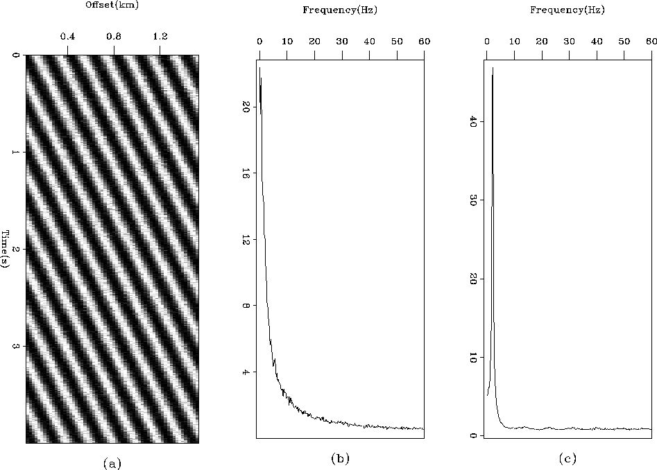
I designed a synthetic case where noise and signal are completely separable. Figure 1a shows the synthetic CMP gather. The data are made of eleven hyperbolic events overlaid by a monochromatic event plus some Gaussian zero mean random noise. H is the velocity stack operator. In the next two sections, I show that the noise filtering is achieved with or without a noise model.

• Filtering with a noise model

The noise model I use is shown in Figure 2a; it contains both the monochromatic event and the random noise. The first parameter I set is the size of the PEF. Because the coherent noise of this dataset was extremely predictable, it seemed that a one dimensional PEF with three coefficients PEF should suffice, but surprisingly, it did not. Figure 2b displays the inverse spectrum of the PEF with three coefficients (a=3,1). Clearly, the estimated noise spectrum does not resemble the coherent noise spectrum in Figure 1b. Using 30 coefficients (a=30,1) significantly improved the matching (Figure 2c). According to this result, I chose a 30 coefficients PEF and iterated for the fitting goal in equation (1).

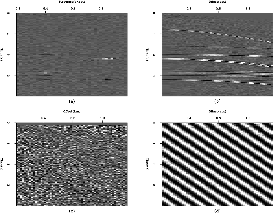
Figures 3a and b show, respectively, the estimated model space after inversion and the reconstructed data. No footprint of the coherent noise appears in either space. In addition, the residual (Figure 3c) is reasonably white, indicating that the inversion algorithm converged. The ``real'' residual in Figure 3d, which measures the difference between the input data and the reconstructed data, displays only the undesirable coherent noise.

 

datasynth
Figure 1 (a) Synthetic data. (b) The amplitude spectrum of the data in panel a.

 

pefs
Figure 2 (a) A coherent noise model used for the synthetic data examples. (b) The inverse spectrum of the PEF estimated from the noise model, with 3 coefficients. (c) The inverse spectrum of the PEF estimated from the noise model, with 30 coefficients.

 

c-synth
Figure 3 Filtering the coherent noise in synthetic data with a noise model. (a) An estimated model space. (b) Reconstructed data using the model space. (c) The weighted residual (${\bf r = A_r(Hm-d)}$) after inversion. (d) The difference between the input data in Figure 1a and the reconstructed data in 3b.

• Filtering without a noise model

The PEF (a=30,1) is now iteratively updated. The first stage of this method is to iterate with no PEF in the fitting goal and then to estimate the PEF after a certain number of iterations from the residual. I iterated 10 times before estimating the filter. Figure 4a displays the residual after 10 iterations and its corresponding spectrum in Figure 4b. As expected, the residual is mostly noise, which makes the first PEF estimation reliable.

In the second stage, after the first PEF calculation, the model space is reset to zero and the conjugate gradient (the iterative solver I used) is restarted. Figure 4c shows the residual after the first iteration. The coherent noise has been properly attenuated. The spectrum in Figure 4d shows almost no trace of the monochromatic event. I then recomputed the PEF after every 10 iterations. 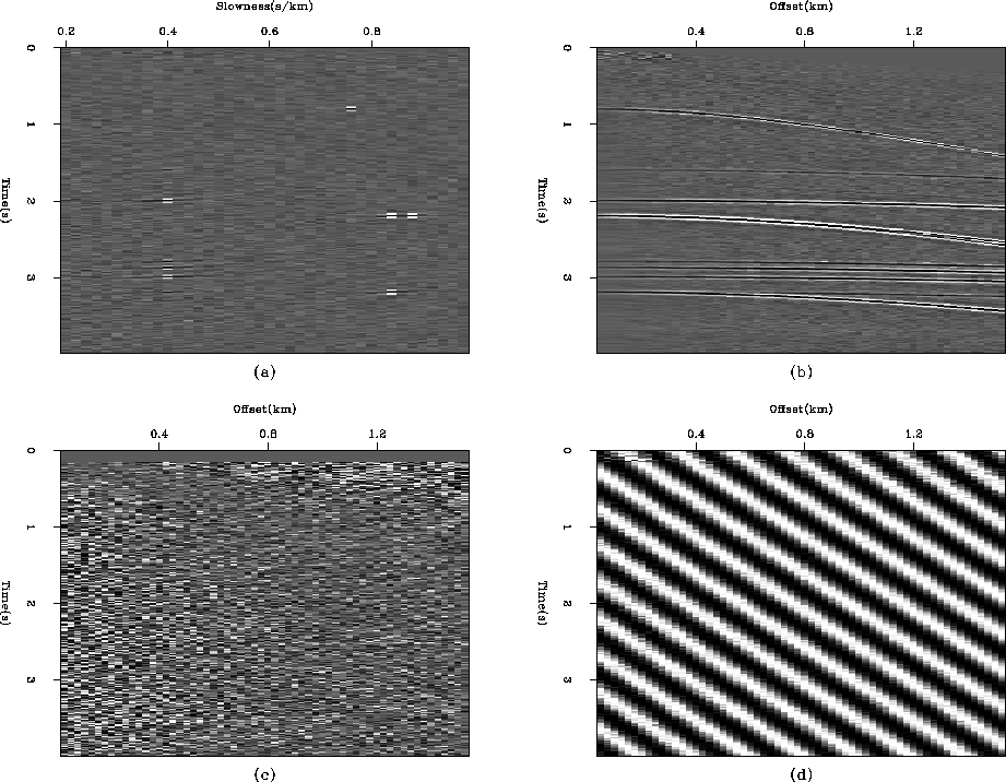The outcome of this process, displayed in Figure 5, is comparable to that in Figure 3.

 

s-synth-rec
Figure 4 (a) The residual of the filtering scheme without a PEF after 10 iterations. (b) The amplitude spectrum of the residual. (c) The residual after the first iteration with a PEF (estimated from the residual in 4a) in the fitting goal. (d) The amplitude spectrum of the residual in 4c. The noise spectrum has vanished from the residual.

 

c-synth-rec
Figure 5 Filtering the coherent noise in synthetic data without a noise model.(a) An estimated model space. (b) Reconstructed data using the model in 5a. (c) The weighted residual (${\bf r = A_r(Hm-d)}$) after inversion. (d) The difference between the input data in Figure 1a and the reconstructed data in 5b.