 |
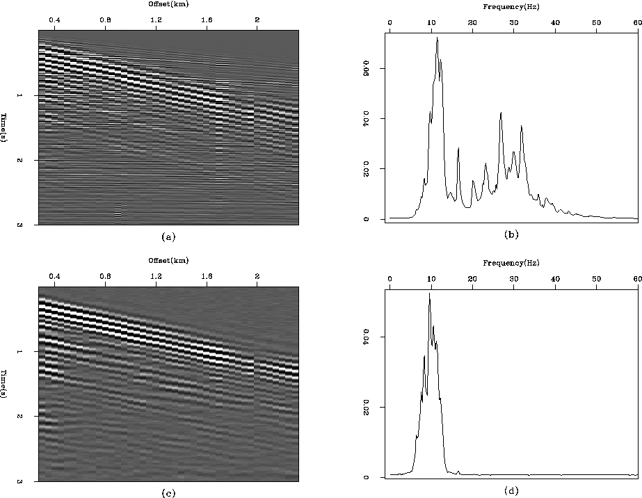
Figure 6 (a) A real CMP gather. (b) The amplitude spectrum of this gather. (c) A noise model obtained by low-passing the data and adding random zero-mean Gaussian noise. (d) The amplitude spectrum of the noise model.
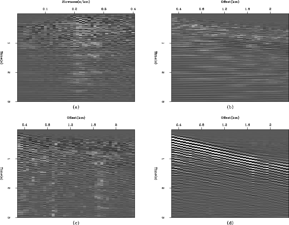
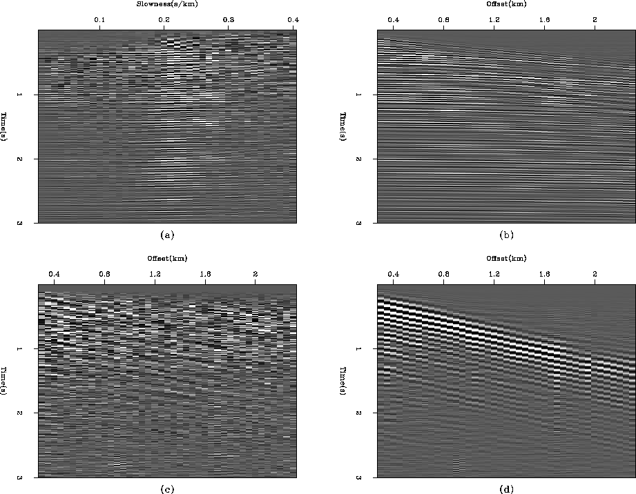
The result of the inversion is displayed in Figure 7. The residual (Figure 7c) is not perfectly white, but the coherent noise has been filtered out. Because the noise model does not incorporate them, the remaining artifacts are the amplitude anomalies.
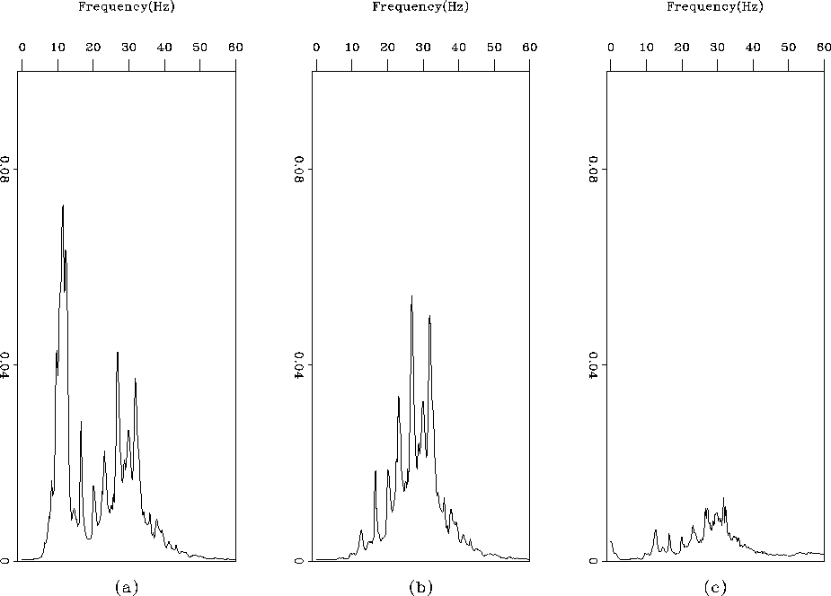
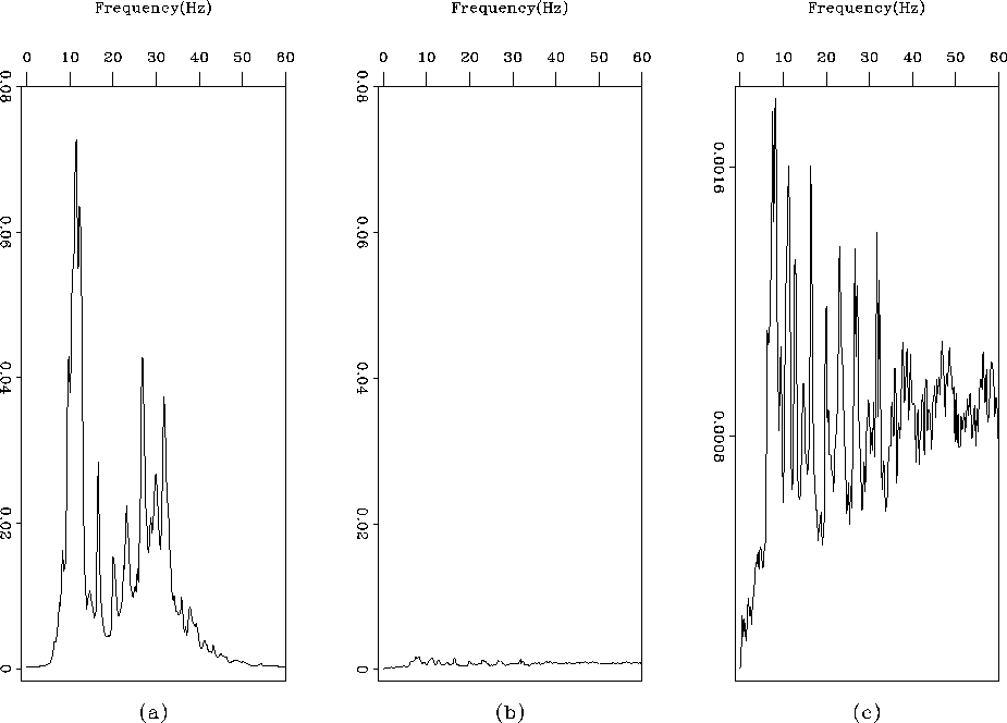
The remaining very weak dipping event in the residual (Figure 7c) needs to be understood. To investigate this issue, I show in Figure 8a the spectrum of the input data; in 8b, the residual before the first iteration; and in 8c, the residual after the inversion ends. We can see that the estimated PEF has eliminated almost all the coherent noise spectrum with a remaining tiny peak at 10 Hertz. As the iterations go on (between Figures 8b and c), the peak does not change in amplitude and becomes relatively more important in the spectrum of the residual, which explains why some coherent information remains in the residual.
The bimodal shape of the spectrum in Figure 8c shows one mode around 10 Hertz for the coherent noise, and one mode around 30 Hertz for the amplitude anomalies. Because I did not reestimate the PEF iteratively, I will not get any whiter residual. I think that a nonstationary PEF would treat the noise more efficiently Guitton et al. (2001). The limited accuracy of the filter I used for the entire residual caused the imperfect attenuation.
 |
 |
![[*]](http://sepwww.stanford.edu/latex2html/movie.gif)
 |
![[*]](http://sepwww.stanford.edu/latex2html/movie.gif)
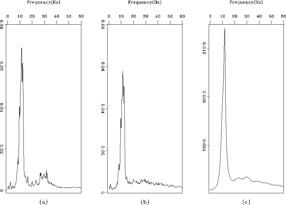
Figures 9a and b shows the spectrum of the residual during the first stage for 10 and 35 iterations. After 10 iterations, I have one peak at 10 Hertz, and a second peak around 30 Hertz. If I estimate a PEF after 10 iterations, it will absorb the two remaining events. The separation tends to be very sensitive to the second peak. Because it overlaps with the signal spectrum, the noise spectrum at 30 Hertz should be avoided in the PEF. I then decided to estimate a PEF after 35 iterations (Figure 9b) since the second peak was considerably attenuated. Figure 9c shows the inverse spectrum of the PEF estimated from the residual with the spectrum in Figure 9b. The main features of the spectrum are correctly absorbed in the filter.
In the second stage of the inversion scheme, I reestimated the PEF only twice during the remaining 38 iterations. There were 73 iterations in total, 35 iterations for the first stage and 38 for the second. Figure 10 displays the final results. In Figure 10c, the residual appears fairly white with little coherent information left. However, there remains a very weak background event with the same slope as the coherent noise I wish to attenuate.
To investigate this problem further, I compute the spectrum of the residual after the inversion ends. Figure 11a shows the spectrum of the input data; Figure 11b, the spectrum of the residual; and Figure 11c, the same spectrum at a smaller scale. The residual looks white with a slightly higher peak at 10 Hertz, which explains the residual in Figure 10c. Nonetheless, the final result is, I think, very satisfactory and compares favorably with the result displayed in Figure 7 when a noise model is known.
To demonstrate the usefulness of a PEF in the fitting goal (equation (1)) further, I computed a comparison, shown in Figure 12, of the normalized objective functions for the iterative scheme with and without a PEF. The PEF clearly improves the optimization.
 |
 |
 |
|
conv
Figure 12 Convergence of the iterative schemes with or without a PEF for seven iterations. The PEF (continuous and dotted lines) allows the best convergence. | 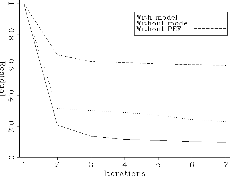 |