


Next: Plane-wave destruction and B-splines
Up: Examples of data regularization
Previous: Gap interpolation
Spitz (1991) popularized the application of
prediction-error filters to regular trace interpolation and showed how
the spatial aliasing restriction can be overcome by scaling the
frequencies of F-X PEFs. An analogous technique for T-X
filters was developed by Claerbout (1992, 1999) and was
applied for 3-D interpolation with non-stationary PEFs by
Crawley (2000). The T-X technique implies
stretching the filter in all directions so that its dip spectrum is
preserved while the coefficients can be estimated at alternating
traces. After the filter is estimated, it is scaled back and used for
interpolating missing traces between the known ones. A similar method
works for finite-difference plane wave destructors, only we need to
take special care to avoid aliased dips at the dip estimation stage.
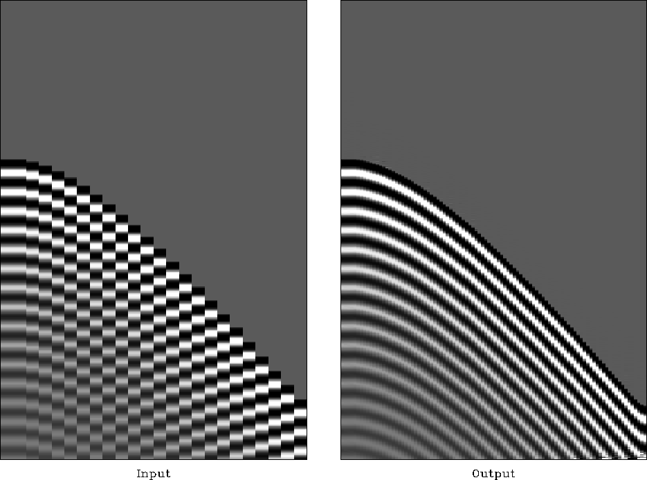
A simple synthetic example of interpolation beyond aliasing is shown
in Figure ![[*]](http://sepwww.stanford.edu/latex2html/cross_ref_motif.gif) . The input data are clearly aliased and
non-stationary. To take the aliasing into account, I estimate the two
dips present in the data with the slope estimation technique of the
previous subsection. The first dip corresponds to the true slope,
while the second dip corresponds to the aliased dip component. In this
example, the true dip is non-negative everywhere and is easily
distinguished from the aliased one. Throwing away the aliased dip and
interpolating intermediate traces with the true dip produces the
accurate interpolation result shown in the right plot of
Figure
. The input data are clearly aliased and
non-stationary. To take the aliasing into account, I estimate the two
dips present in the data with the slope estimation technique of the
previous subsection. The first dip corresponds to the true slope,
while the second dip corresponds to the aliased dip component. In this
example, the true dip is non-negative everywhere and is easily
distinguished from the aliased one. Throwing away the aliased dip and
interpolating intermediate traces with the true dip produces the
accurate interpolation result shown in the right plot of
Figure ![[*]](http://sepwww.stanford.edu/latex2html/cross_ref_motif.gif) .
.
aliasp2
Figure 13 Synthetic example of
interpolation beyond aliasing with plane-wave destructor filters.
Left: input aliased data, right: interpolation output.


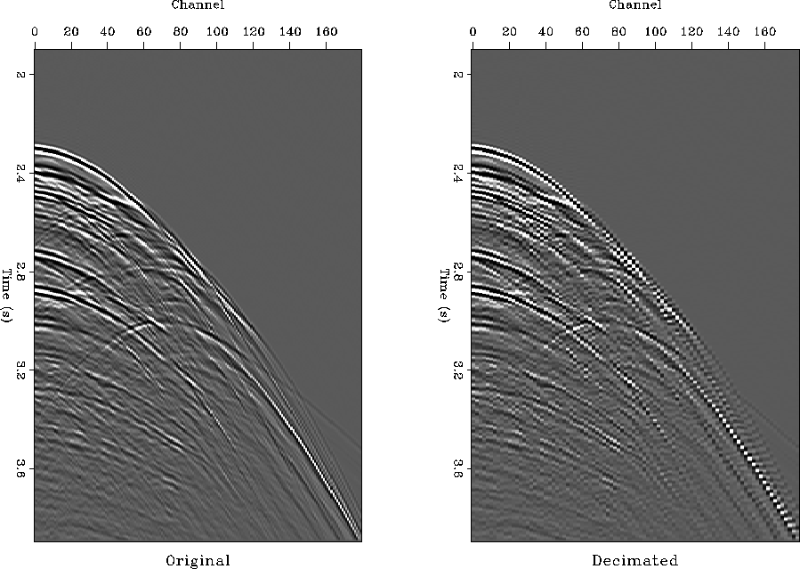
Figure ![[*]](http://sepwww.stanford.edu/latex2html/cross_ref_motif.gif) shows a marine 2-D shot gather from a deep
water Gulf of Mexico survey before and after subsampling in the offset
direction. The data are similar to those used by
Crawley (2000). The shot gather has long-period
multiples and complicated diffraction events caused by a salt body.
The amplitudes of the hyperbolic events are not as uniformly
distributed as in the synthetic case of Figure
shows a marine 2-D shot gather from a deep
water Gulf of Mexico survey before and after subsampling in the offset
direction. The data are similar to those used by
Crawley (2000). The shot gather has long-period
multiples and complicated diffraction events caused by a salt body.
The amplitudes of the hyperbolic events are not as uniformly
distributed as in the synthetic case of Figure ![[*]](http://sepwww.stanford.edu/latex2html/cross_ref_motif.gif) .
Subsampling by a factor of two (the right plot in
Figure
.
Subsampling by a factor of two (the right plot in
Figure ![[*]](http://sepwww.stanford.edu/latex2html/cross_ref_motif.gif) ) causes a clearly visible aliasing in the
steeply dipping events. The goal of the experiment is to interpolate
the missing traces in the subsampled data and to compare the result
with the original gather shown in the left plot of
Figure
) causes a clearly visible aliasing in the
steeply dipping events. The goal of the experiment is to interpolate
the missing traces in the subsampled data and to compare the result
with the original gather shown in the left plot of
Figure ![[*]](http://sepwww.stanford.edu/latex2html/cross_ref_motif.gif) .
.
sean2
Figure 14 2-D marine shot gather. Left:
original. Right: subsampled by a factor of two in the offset
direction.


A straightforward application of the dip estimation
equations (![[*]](http://sepwww.stanford.edu/latex2html/cross_ref_motif.gif) -
-![[*]](http://sepwww.stanford.edu/latex2html/cross_ref_motif.gif) ) applied to aliased data can
easily lead to erroneous aliased dip estimation. In order to avoid
this problem, I chose a slightly more complex strategy. The algorithm for trace
interpolation of aliased data consists of the following steps:
) applied to aliased data can
easily lead to erroneous aliased dip estimation. In order to avoid
this problem, I chose a slightly more complex strategy. The algorithm for trace
interpolation of aliased data consists of the following steps:
- 1.
- Applying Claerbout's T-X methodology, stretch a two-dip
plane-wave destructor filter and estimate the dips from decimated
data.
- 2.
- The second estimated dip will be degraded by aliasing. Ignore
this initial second-dip estimate.
- 3.
- Estimate the second dip component again by fixing the first dip
component and using it as the initial estimate of the second
component. This trick prevents the nonlinear estimation algorithm
from picking the wrong (aliased) dip in the data.
- 4.
- Downscale the estimated two-dip filter and use it for
interpolating missing traces.
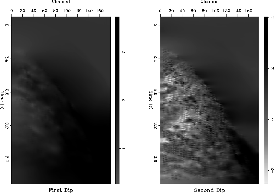
The two estimated dip components are shown in
Figure ![[*]](http://sepwww.stanford.edu/latex2html/cross_ref_motif.gif) . The first component contains only positive
dips. The second component coincides with the first one in the areas
where only a single dip is present in the data. In other areas, it
picks the complementary dip, which has a negative value for
back-dipping hyperbolic diffractions.
sean2-dip
. The first component contains only positive
dips. The second component coincides with the first one in the areas
where only a single dip is present in the data. In other areas, it
picks the complementary dip, which has a negative value for
back-dipping hyperbolic diffractions.
sean2-dip
Figure 15 Two components of the
estimated dip field for the decimated 2-D marine shot gather.


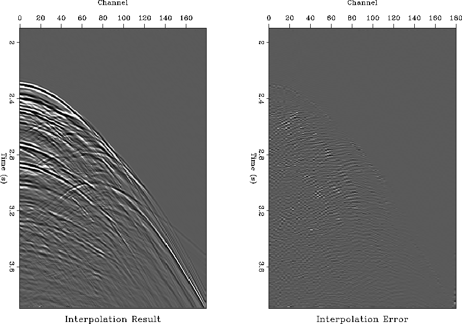
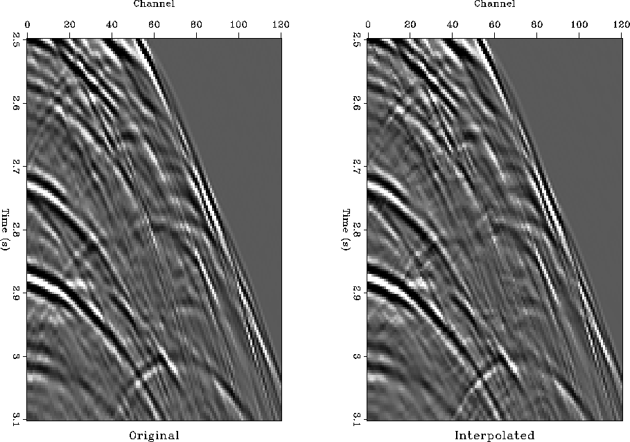
Figure ![[*]](http://sepwww.stanford.edu/latex2html/cross_ref_motif.gif) shows the interpolation result and the
difference between the interpolated traces and the original traces,
plotted at the same clip value. The method succeeded in the sense that
it is impossible to distinguish interpolated traces from the
interpolation result alone. However, it is not ideal, because some of
the original energy is missing in the output. A close-up comparison
between the original and the interpolated traces in
Figure
shows the interpolation result and the
difference between the interpolated traces and the original traces,
plotted at the same clip value. The method succeeded in the sense that
it is impossible to distinguish interpolated traces from the
interpolation result alone. However, it is not ideal, because some of
the original energy is missing in the output. A close-up comparison
between the original and the interpolated traces in
Figure ![[*]](http://sepwww.stanford.edu/latex2html/cross_ref_motif.gif) shows that imperfection in more detail.
Some of the steepest events in the middle of the section are poorly
interpolated, and in some of the other places, the second dip
component is continued instead of the first one.
shows that imperfection in more detail.
Some of the steepest events in the middle of the section are poorly
interpolated, and in some of the other places, the second dip
component is continued instead of the first one.
sean2-int
Figure 16 Left: 2-D marine shot
gather after trace interpolation. Right: Difference between the
interpolated and the original gather.


 sean2-close
Figure 17 Close-up comparison of
the interpolated (right) and the original data (left).
![[*]](http://sepwww.stanford.edu/latex2html/movie.gif)


One could improve the interpolation result considerably by including
another dimension. To achieve a better result, we can use a pair of
plane-wave destructors, one predicting local plane waves in the offset
direction and the other predicting local plane waves in the shot
direction.


Next: Plane-wave destruction and B-splines
Up: Examples of data regularization
Previous: Gap interpolation
Stanford Exploration Project
12/28/2000
![[*]](http://sepwww.stanford.edu/latex2html/cross_ref_motif.gif) . The input data are clearly aliased and
non-stationary. To take the aliasing into account, I estimate the two
dips present in the data with the slope estimation technique of the
previous subsection. The first dip corresponds to the true slope,
while the second dip corresponds to the aliased dip component. In this
example, the true dip is non-negative everywhere and is easily
distinguished from the aliased one. Throwing away the aliased dip and
interpolating intermediate traces with the true dip produces the
accurate interpolation result shown in the right plot of
Figure
. The input data are clearly aliased and
non-stationary. To take the aliasing into account, I estimate the two
dips present in the data with the slope estimation technique of the
previous subsection. The first dip corresponds to the true slope,
while the second dip corresponds to the aliased dip component. In this
example, the true dip is non-negative everywhere and is easily
distinguished from the aliased one. Throwing away the aliased dip and
interpolating intermediate traces with the true dip produces the
accurate interpolation result shown in the right plot of
Figure ![[*]](http://sepwww.stanford.edu/latex2html/cross_ref_motif.gif) .
.
![[*]](http://sepwww.stanford.edu/latex2html/movie.gif)