![[*]](http://sepwww.stanford.edu/latex2html/cross_ref_motif.gif) as a simple case of data regularization
when the input data are already binned to regular grid locations but
with remaining uncovered gaps.
as a simple case of data regularization
when the input data are already binned to regular grid locations but
with remaining uncovered gaps.
Missing-data interpolation was introduced in
Chapter ![[*]](http://sepwww.stanford.edu/latex2html/cross_ref_motif.gif) as a simple case of data regularization
when the input data are already binned to regular grid locations but
with remaining uncovered gaps.
as a simple case of data regularization
when the input data are already binned to regular grid locations but
with remaining uncovered gaps.
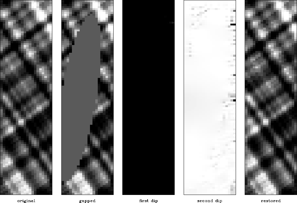
Figure ![[*]](http://sepwww.stanford.edu/latex2html/cross_ref_motif.gif) shows a simple synthetic example of gap
interpolation from Claerbout (1999). The input data has a large
elliptic gap cut out in a two plane-wave model. I estimate both dip
components from the input data by using the method of
equations (
shows a simple synthetic example of gap
interpolation from Claerbout (1999). The input data has a large
elliptic gap cut out in a two plane-wave model. I estimate both dip
components from the input data by using the method of
equations (![[*]](http://sepwww.stanford.edu/latex2html/cross_ref_motif.gif) -
-![[*]](http://sepwww.stanford.edu/latex2html/cross_ref_motif.gif) ). The initial values for the
two local dips were 1 and 0, and the estimated values are close to the
true dips of 2 and -1 (the third and fourth plots in
Figure
). The initial values for the
two local dips were 1 and 0, and the estimated values are close to the
true dips of 2 and -1 (the third and fourth plots in
Figure ![[*]](http://sepwww.stanford.edu/latex2html/cross_ref_motif.gif) .) Although the estimation program does not make
any assumption about dip being constant, it correctly estimates nearly
constant values with the help of regularization
equations (
.) Although the estimation program does not make
any assumption about dip being constant, it correctly estimates nearly
constant values with the help of regularization
equations (![[*]](http://sepwww.stanford.edu/latex2html/cross_ref_motif.gif) -
-![[*]](http://sepwww.stanford.edu/latex2html/cross_ref_motif.gif) ). The rightmost plot in
Figure
). The rightmost plot in
Figure ![[*]](http://sepwww.stanford.edu/latex2html/cross_ref_motif.gif) shows the result of gap interpolation with a
two-plane local plane-wave destructor. The result is nearly ideal and
compares favorably with the analogous result of the T-X PEF
technique Claerbout (1999).
shows the result of gap interpolation with a
two-plane local plane-wave destructor. The result is nearly ideal and
compares favorably with the analogous result of the T-X PEF
technique Claerbout (1999).
 |
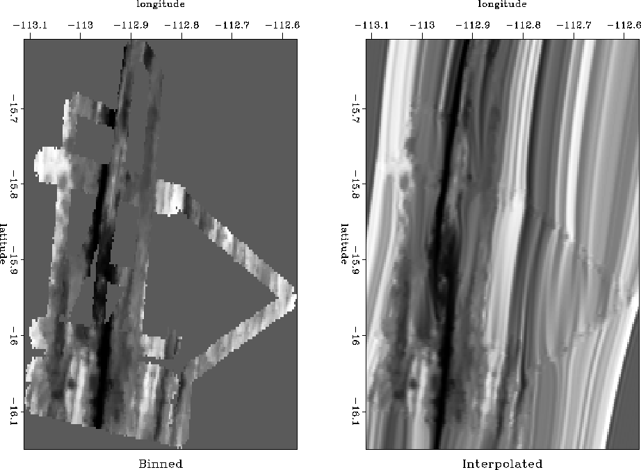
Figure ![[*]](http://sepwww.stanford.edu/latex2html/cross_ref_motif.gif) is another benchmark gap interpolation example
from Claerbout (1999), already featured in Chapter
is another benchmark gap interpolation example
from Claerbout (1999), already featured in Chapter ![[*]](http://sepwww.stanford.edu/latex2html/cross_ref_motif.gif) (Figures
(Figures ![[*]](http://sepwww.stanford.edu/latex2html/cross_ref_motif.gif) -
-![[*]](http://sepwww.stanford.edu/latex2html/cross_ref_motif.gif) ). The data are
ocean-depth measurements from one day SeaBeam acquisition. The data
after normalized binning are shown in the left plot of
Figure
). The data are
ocean-depth measurements from one day SeaBeam acquisition. The data
after normalized binning are shown in the left plot of
Figure ![[*]](http://sepwww.stanford.edu/latex2html/cross_ref_motif.gif) . From the known part of the data, we can
partially see a certain elongated and faulted structure on the ocean
floor created by fractures around an ocean ridge. Estimating a
smoothed dominant dip in the data and interpolating with the
plane-wave destructor filters produces the image in the right plot of
Figure
. From the known part of the data, we can
partially see a certain elongated and faulted structure on the ocean
floor created by fractures around an ocean ridge. Estimating a
smoothed dominant dip in the data and interpolating with the
plane-wave destructor filters produces the image in the right plot of
Figure ![[*]](http://sepwww.stanford.edu/latex2html/cross_ref_motif.gif) . The V-shaped acquisition pattern is somewhat
visible in the interpolation result, which might indicate the presence
of a fault. Otherwise, the result is both visually pleasing and in
full agreement with the input data. Clapp (2000b)
uses the same data example to obtain multiple statistically equivalent
realizations of the interpolated data.
. The V-shaped acquisition pattern is somewhat
visible in the interpolation result, which might indicate the presence
of a fault. Otherwise, the result is both visually pleasing and in
full agreement with the input data. Clapp (2000b)
uses the same data example to obtain multiple statistically equivalent
realizations of the interpolated data.
 |
![[*]](http://sepwww.stanford.edu/latex2html/movie.gif)
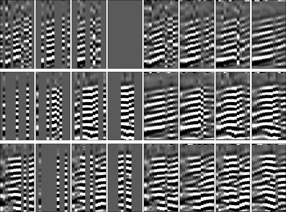
A 3-D interpolation example is shown in Figure ![[*]](http://sepwww.stanford.edu/latex2html/cross_ref_motif.gif) . The
input data resulted from a passive seismic experiment
Cole (1995) and originally contained many gaps because of
instrument failure. I interpolated the 3-D gaps with a pair of two
orthogonal plane-wave destructors in the manner proposed by
Schwab and Claerbout (1995) for T-X prediction filters. The
interpolation result shows a visually pleasing continuation of locally
plane events through the gaps. It compares favorably with an analogous
result of a stationary T-X PEF.
. The
input data resulted from a passive seismic experiment
Cole (1995) and originally contained many gaps because of
instrument failure. I interpolated the 3-D gaps with a pair of two
orthogonal plane-wave destructors in the manner proposed by
Schwab and Claerbout (1995) for T-X prediction filters. The
interpolation result shows a visually pleasing continuation of locally
plane events through the gaps. It compares favorably with an analogous
result of a stationary T-X PEF.
 |
![[*]](http://sepwww.stanford.edu/latex2html/movie.gif)
We can conclude that plane-wave destructors provide an effective method of gap filling and missing-data interpolation.